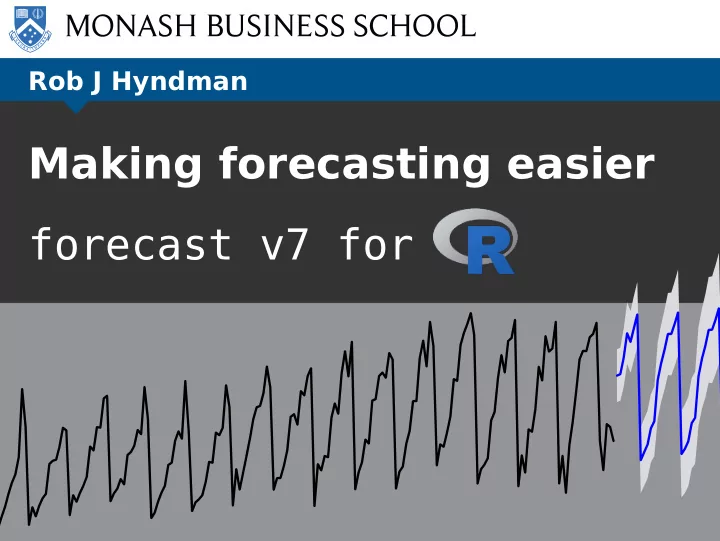
Making forecasting easier forecast v7 for Outline 1 Motivation - PowerPoint PPT Presentation

Rob J Hyndman Making forecasting easier forecast v7 for

Outline 1 Motivation and history 2 Automatic forecasting in R 3 ggplot2 graphics 4 Bias adjustment Making forecasting easier Motivation and history 2

Motivation Making forecasting easier Motivation and history 3

Motivation Making forecasting easier Motivation and history 3

Motivation Making forecasting easier Motivation and history 3

Motivation Making forecasting easier Motivation and history 3

Motivation Making forecasting easier Motivation and history 3

Motivation Common in business to have thousands of 1 products that need forecasting at least monthly. Forecasts are often required by people who are 2 untrained in time series analysis. Specifications Automatic forecasting algorithms must: ➥ determine an appropriate time series model; ➥ estimate the parameters; ➥ compute the forecasts with prediction intervals. Making forecasting easier Motivation and history 4

Motivation Common in business to have thousands of 1 products that need forecasting at least monthly. Forecasts are often required by people who are 2 untrained in time series analysis. Specifications Automatic forecasting algorithms must: ➥ determine an appropriate time series model; ➥ estimate the parameters; ➥ compute the forecasts with prediction intervals. Making forecasting easier Motivation and history 4

Forecast package history Pre 2003 Collection of functions used for consulting projects July/August 2003 ets and thetaf added August 2006 v1.0 available on CRAN May 2007 auto.arima added July 2008 JSS paper (Hyndman & Khandakar) September 2009 v2.0. Unbundled. May 2010 arfima added Feb/March 2011 tslm , stlf , naive , snaive added August 2011 v3.0. Box Cox transformations added December 2011 tbats added April 2012 Package moved to github November 2012 v4.0. nnetar added June 2013 Major speed-up of ets January 2014 v5.0. tsoutliers and tsclean added May 2015 v6.0. Added several new plots December 2015 264,000 package downloads in one month! February 2016 v7.0. Added ggplot2 graphics & bias adjustment Making forecasting easier Motivation and history 5

Outline 1 Motivation and history 2 Automatic forecasting in R 3 ggplot2 graphics 4 Bias adjustment Making forecasting easier Automatic forecasting in R 6

Automatic methods in forecast package Automatic model Automatic forecasting selection auto.arima + forecast forecast.ts ets + forecast stlf tbats + forecast thetaf bats + forecast dshw, hw, holt, ses arfima + forecast splinef ar + forecast rwf, naive nnetar + forecast croston stlm + forecast All produce an object of class “forecast” Making forecasting easier Automatic forecasting in R 7

ets algorithm in R Based on Hyndman, Koehler, Snyder & Grose (IJF 2002): For each model, optimize parameters and initial values of underlying state space model using MLE. Select best method using AICc. Produce forecasts and prediction intervals using best method. Making forecasting easier Automatic forecasting in R 8

ets algorithm in R Based on Hyndman, Koehler, Snyder & Grose (IJF 2002): For each model, optimize parameters and initial values of underlying state space model using MLE. Select best method using AICc. Produce forecasts and prediction intervals using best method. Making forecasting easier Automatic forecasting in R 8

ets algorithm in R Based on Hyndman, Koehler, Snyder & Grose (IJF 2002): For each model, optimize parameters and initial values of underlying state space model using MLE. Select best method using AICc. Produce forecasts and prediction intervals using best method. Making forecasting easier Automatic forecasting in R 8

Exponential smoothing Forecasts from ETS(M,A,N) 600 500 400 300 1960 1970 1980 1990 2000 2010 Making forecasting easier Automatic forecasting in R 9

Exponential smoothing Forecasts from ETS(M,A,N) 600 fit <- ets(livestock) fcast <- forecast(fit) plot(fcast) 500 400 300 1960 1970 1980 1990 2000 2010 Making forecasting easier Automatic forecasting in R 10

Exponential smoothing Forecasts from ETS(M,Ad,M) 1.4 1.2 1.0 0.8 0.6 0.4 1995 2000 2005 2010 Making forecasting easier Automatic forecasting in R 11

Exponential smoothing Forecasts from ETS(M,Ad,M) fit <- ets(h02) 1.4 fcast <- forecast(fit) 1.2 plot(fcast) 1.0 0.8 0.6 0.4 1995 2000 2005 2010 Making forecasting easier Automatic forecasting in R 12

auto.arima algorithm in R Based on Hyndman and Khandakar (JSS 2008): Select no. differences via unit root tests. Use stepwise search to traverse model space, starting with a simple model and considering nearby variants. For each model, optimize parameters using MLE. Select best method using AICc. Produce forecasts and prediction intervals using best method. Making forecasting easier Automatic forecasting in R 13

auto.arima algorithm in R Based on Hyndman and Khandakar (JSS 2008): Select no. differences via unit root tests. Use stepwise search to traverse model space, starting with a simple model and considering nearby variants. For each model, optimize parameters using MLE. Select best method using AICc. Produce forecasts and prediction intervals using best method. Making forecasting easier Automatic forecasting in R 13

auto.arima algorithm in R Based on Hyndman and Khandakar (JSS 2008): Select no. differences via unit root tests. Use stepwise search to traverse model space, starting with a simple model and considering nearby variants. For each model, optimize parameters using MLE. Select best method using AICc. Produce forecasts and prediction intervals using best method. Making forecasting easier Automatic forecasting in R 13

auto.arima algorithm in R Based on Hyndman and Khandakar (JSS 2008): Select no. differences via unit root tests. Use stepwise search to traverse model space, starting with a simple model and considering nearby variants. For each model, optimize parameters using MLE. Select best method using AICc. Produce forecasts and prediction intervals using best method. Making forecasting easier Automatic forecasting in R 13

auto.arima algorithm in R Based on Hyndman and Khandakar (JSS 2008): Select no. differences via unit root tests. Use stepwise search to traverse model space, starting with a simple model and considering nearby variants. For each model, optimize parameters using MLE. Select best method using AICc. Produce forecasts and prediction intervals using best method. Making forecasting easier Automatic forecasting in R 13

Auto ARIMA Forecasts from ARIMA(0,1,0) with drift 550 500 450 400 350 300 250 1960 1970 1980 1990 2000 2010 Making forecasting easier Automatic forecasting in R 14

Auto ARIMA Forecasts from ARIMA(0,1,0) with drift fit <- auto.arima(livestock) 550 fcast <- forecast(fit) 500 plot(fcast) 450 400 350 300 250 1960 1970 1980 1990 2000 2010 Making forecasting easier Automatic forecasting in R 15

Auto ARIMA Forecasts from ARIMA(3,1,3)(0,1,1)[12] 1.4 1.2 1.0 0.8 0.6 0.4 1995 2000 2005 2010 Making forecasting easier Automatic forecasting in R 16

Auto ARIMA Forecasts from ARIMA(3,1,3)(0,1,1)[12] 1.4 fit <- auto.arima(h02) fcast <- forecast(fit) 1.2 plot(fcast) 1.0 0.8 0.6 0.4 1995 2000 2005 2010 Making forecasting easier Automatic forecasting in R 17

TBATS model TBATS T rigonometric terms for seasonality B ox-Cox transformations for heterogeneity A RMA errors for short-term dynamics T rend (possibly damped) S easonal (including multiple and non-integer periods) Automatic algorithm described in De Livera, Hyndman and Snyder (JASA 2011). Making forecasting easier Automatic forecasting in R 18

Examples Forecasts from TBATS(1, {0,0}, 1, {<52.1785714285714,9>}) fit <- tbats(gas) 10 fcast <- forecast(fit) plot(fcast) 9 8 7 1995 2000 2005 Making forecasting easier Automatic forecasting in R 19

Examples Forecasts from TBATS(0.607, {0,0}, −, {<169,5>, <845,4>}) fit <- tbats(callcentre) 500 fcast <- forecast(fit) plot(fcast) 400 300 200 100 0 2005 2010 2015 2020 2025 2030 2035 Making forecasting easier Automatic forecasting in R 20

Outline 1 Motivation and history 2 Automatic forecasting in R 3 ggplot2 graphics 4 Bias adjustment Making forecasting easier ggplot2 graphics 21

ggplot2 graphics Internet Usage per Minute plot(WWWusage, xlab="Minutes", ylab="Internet users", 200 main="Internet Usage per Minute") Internet users 150 100 0 20 40 60 80 100 Minutes Making forecasting easier ggplot2 graphics 22

ggplot2 graphics Internet Usage per Minute autoplot(WWWusage, xlab="Minutes", ylab="Internet users", main="Internet Usage per Minute") 200 Internet users 160 120 80 0 25 50 75 100 Minutes Making forecasting easier ggplot2 graphics 23

ggplot2 graphics Forecasts from ETS(A,Ad,N) 300 autoplot(forecast(WWWusage)) 250 level 200 80 y 95 150 100 0 30 60 90 Time Making forecasting easier ggplot2 graphics 24