main twist today: separate DC power flow : ( Y ) = 0 , v = 1 , & - PowerPoint PPT Presentation
Power flow equations Fast power system analysis via implicit Basic ingredients in an n -bus power system linearization of the power flow manifold complex bus voltage u h = v h e j h C injected complex power s h = p h + j q h Allerton
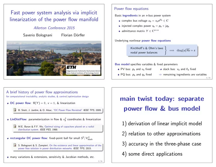
Power flow equations Fast power system analysis via implicit Basic ingredients in an n -bus power system linearization of the power flow manifold complex bus voltage u h = v h e j θ h ∈ C injected complex power s h = p h + j q h Allerton Conference 2015 admittance matrix Y ∈ C n × n Saverio Bolognani Florian D¨ orfler Underlying nonlinear power flow equations � Kirchhoff’s & Ohm’s laws = ⇒ diag ( u ) Yu = s nodal power balances Bus model specifies variables & fixed parameters PV bus: p h and v h fixed slack bus: v h and θ h fixed PQ bus: p h and q h fixed ⇒ remaining ingredients are variables 2 / 16 A brief history of power flow approximations for computational tractability, analytic studies, & control/optimization design main twist today: separate DC power flow : ℜ ( Y ) = 0 , v = 1 , & linearization power flow & bus model B. Stott, J. Jardim, & O. Alsac, “DC Power Flow Revisited” IEEE TPS , 2009. LinDistFlow : parameterization in flow & v 2 h coordinates & linearization 1) derivation of linear implicit model M.E. Baran & F.F. Wu, Optimal sizing of capacitors placed on a radial distribution system. IEEE PES , 1988. 2) relation to other approximations rectangular DC power flow : fixed-point ball for small S 2 / V 2 slack 3) accuracy in the three-phase case S. Bolognani & S. Zampieri, On the existence and linear approximation of the power flow solution in power distribution networks. IEEE TPS , 2015. 4) some direct applications many variations & extensions, sensitivity & Jacobian methods, etc. 3 / 16
Linear implicit model & its advantages The power flow manifold & linear tangent approximation today consider all of x = ( v , θ, p , q ) as variables 1.2 1 node 1 node 2 implicit model for power flow manifold: F ( x ) = 0 0.8 v 2 0.6 linear approximant at x ∗ is tangent plane: A ( x − x ∗ ) = 0 y = 0 . 4 − 0 . 8 j 0.4 v 1 = 1 , θ 1 = 0 v 2 , θ 2 1 p 1 , q 1 p 2 , q 2 Advantages of linear implicit model: 0.5 2 ◮ sparsity 1 0 0.5 q 2 0 -0.5 p 2 1 power flow manifold: F ( x ) = 0 ⇒ tractable for applications with 1 high computational burden � theta 0 2 normal space spanned by ∂ F ( x ) � x ∗ = A T ◮ structure-preserving 1.4 � ∂ x 1.2 -1 ⇒ prior for distributed control, 1 v 2 3 tangent space at x ∗ : A ( x − x ∗ ) = 0 1.5 optimization, estimation, etc. 0.8 -2 1 -2.5 -2 0.6 -1.5 -1 0.5 -0.5 -2 ◮ geometric methods 0 -1 -1 q 0.5 0 1 1 4 accuracy depends on curvature ∂ 2 F ( x ) 2 p -0.5 0 0 ∂ x 2 -0.5 0.5 two-bus example q 2 1 ⇒ explicitly require tangent planes p 2 -1 1.5 4 / 16 5 / 16 Closer look at implicit formulae A ( x − x ∗ ) = 0 �� � diag (cos θ ∗ ) − diag ( v ∗ ) diag (sin θ ∗ ) �� � � diag Yu ∗ � + � diag u ∗ � N � Y � · diag (sin θ ∗ ) diag ( v ∗ ) diag (cos θ ∗ ) � �� � � �� � � �� � . . . appears shunt loads lossy DC flow rotation × scaling at operating point � v − v ∗ � � p − p ∗ � cumbersome × = θ − θ ∗ q − q ∗ � �� � at first glance deviation variables � I � 0 where N = is complex conjugate in real coordinates 0 − I � ℜ ( A ) � −ℑ ( A ) and � A � = is complex rotation in real coordinates. ℑ ( A ) ℜ ( A ) 6 / 16
Special cases reveal some old friends I Special cases reveal some old friends II flat-voltage/0-injection point: x ∗ = ( v ∗ , θ ∗ , p ∗ , q ∗ ) = ( 1 , 0 , 0 , 0 ) flat-voltage/0-injection point: x ∗ = ( v ∗ , θ ∗ , p ∗ , q ∗ ) = ( 1 , 0 , 0 , 0 ) � ℜ ( Y ) � � v � � p � −ℑ ( Y ) ⇒ rectangular coord. ⇒ rectangular DC flow [S. Bolognani & S. Zampieri, 2015] ⇒ implicit linearization: = −ℑ ( Y ) ℜ ( Y ) θ q nonlinear change to quadratic coordinates from v h to v 2 is linear coupled power flow [D. Deka, S. Backhaus, & M. Chertkov, 2015] h ⇒ linearization gives (non-radial) LinDistFlow [M.E. Baran & F.F. Wu, 1988] ⇒ ℜ ( Y ) = 0 gives DC power flow: −ℑ ( Y ) θ = p and −ℑ ( Y ) v = q 1.4 1.5 1.3 power flow manifold 1 1.2 power flow manifold 1.1 0.5 linear approximation 1 linear coupled power flow v 2 p 2 0 0.9 DC power flow approximation linear approximation 0.8 -0.5 (neglects PV coupling) in quadratic coordinates 0.7 -1 2 0.6 0.6 -1 1 0.8 0 1.5 1 0 0.5 1 1 0 -1 -0.5 1.2 2 -1 p 2 v 2 1.4 -2 ! 2 7 / 16 q 2 8 / 16 Extensions to more general models Bus device models , e.g., PQ bus s h = p h + j q h = const . ⇒ implicit constraint g ( x ) = 0 & can be absorbed in F ( x ) = 0 Exponential load models s h = const . · v const . h so all standard approximations ⇒ can be handled analogously are included as special cases Unbalanced three-phase grids with basic ingredients h ] T ∈ C 3 complex voltage u h = [ u a h u b h u c similar definitions for other quantities ⇒ all previous results can be analogously re-derived Matlab/Octave code available: https://github.com/saveriob/1ACPF 9 / 16
Accuracy illustrated with unbalanced three-phase IEEE13 a glorified & highly accurate linearization . . . so what? ——– some direct applications ◦ exact solution ⋆ linear implicit model 10 / 16 Fast scenario-based decision making under uncertainties Distributed online optimization on power flow manifold with Adrian Hauswirth & Gabriela Hug (ETH Z¨ urich) Example: feasible region for distribution network operation � � � � Prob { x exo ∈ X exo gradient of cost x dec : F ( x ) = 0 & Vx ≤ w } ≥ 1 − ε Objective Value [$] 810 realized cost tangent space 800 lower bound ���� � �� � � �� � � �� � � �� � projected 790 operating actuation random loads power flow constraints chance 780 gradient point 770 760 750 740 new operating point Scenario-based approach: 730 0 50 100 150 200 250 300 350 400 450 500 sample x exo variables & build Voltage Levels [p.u.] deterministic constraints 1.06 power flow manifold V tab 1.05 ⇒ decision x dec is feasible 1.04 p rojected gradient step with high probability for 1.03 (distributed algorithm) sufficiently many samples 1.02 injections measurements 1.01 0 50 100 150 200 250 300 350 400 450 500 P 671 new operating point applied to optimal voltage control in IEEE 30 bus grid (physical system) S. Bolognani & F. D¨ orfler. Fast scenario-based decision making in unbalanced distribution networks. Power Systems Computation Conference (PSCC) , June 2016. 11 / 16 12 / 16
Recommend
More recommend
Explore More Topics
Stay informed with curated content and fresh updates.
