Magnetism at finite temperature Claudine Lacroix, Insitut Nel, CNRS - PowerPoint PPT Presentation

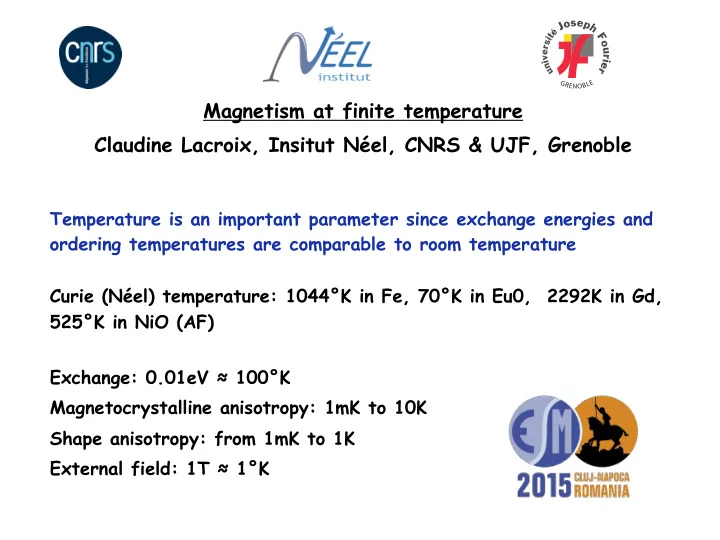
Magnetism at finite temperature Claudine Lacroix, Insitut Néel, CNRS & UJF, Grenoble Temperature is an important parameter since exchange energies and ordering temperatures are comparable to room temperature Curie (Néel) temperature: 1044°K in Fe, 70°K in Eu0, 2292K in Gd, 525°K in NiO (AF) Exchange: 0.01eV ≈ 100°K Magnetocrystalline anisotropy: 1mK to 10K Shape anisotropy: from 1mK to 1K External field: 1T ≈ 1°K

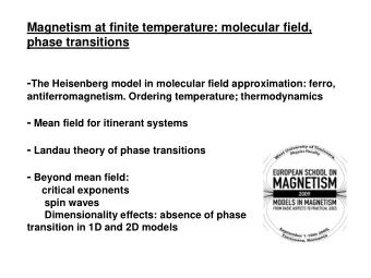
Outline - The Heisenberg model in molecular field approximation - Landau theory of phase transitions - Beyond mean field: - Magnons (spin waves) - Ginzburg-Landau theory - Critical behavior - Role of dimensionality: 1D and 2D systems

Outline - The Heisenberg model in molecular field approximation - Landau theory of phase transitions - Beyond mean field: - Magnons (spin waves) - Ginzburg-Landau theory - Critical behavior - Role of dimensionality: 1D and 2D systems

Various microscopic mecanisms for exchange interactions in solids: - Localized / itinerant spin systems - Short / long range - Ferro or antiferro Various types of ordered magnetic structures: Type of magnetic order depends on the interactions Also spin glasses, spin liquids… : no long range magnetic order

The various exchange mecanisms can usually be described by an effective exchange hamiltonian: Heisenberg model J ij can be long or short range, positive or negative : classical (vector) or quantum spin It is an interaction between spins: if the magnetic moment is given by J instead of S (J=L+S), interaction can be rewritten as: If J ¡= ¡L+S , and L+2S ¡= ¡g J ¡J , then, S ¡= ¡(g-­‑1)J ¡ and I ij ¡= ¡(g-­‑1) 2 ¡J ij ¡ In this lecture: no anisotropy effect K coefficients vary with T as M n

What is mean field approximation ? one moment in a magnetic field H ext : Where the function g is - the Brillouin function (quantum case) - or the Langevin function (classical spins) Heisenberg model: Main assumption: is replaced by its average (similar to molecular field, or Hartree-Fock approximation)

J ij field acting on due to the other spins : If there is also an external field: Initial problem: many-body system of interacting spins New problem: collection of spins in static local magnetic field

Mean field approximation The field created by the neighbors is static; i.e. all thermal and quantum fluctuations are neglected. When fluctuations are small, it is a good approximation. Fluctuations are large - at high temperature: near T c (critical behavior) and above T c (paramagnetic fluctuations) - in low dimensional systems (1D, 2D) - Small spin value (quantum fluctuations):effect of spin waves is more important for small S-value If fluctuations are large, corrections to mean field are important

The molecular field approximation Each magnetic moment is in an effective field external field + field created by the neighboring moments Local magnetization: ( g is Brillouin or Langevin function) Set of coupled equations to determine on each site In a ferromagnet, it becomes simple since is uniform :

New problem: each spin is in a local field that depands on surroundings Hypothesis on the nature of ground state: Ferromagnetic state: (uniform solution) 2 sublattices AF Helimagnets: Receipe: for each solution, solve the selfconsistent equations, calculate S, calculate the corresponding free energy, compare the energy of the various solutions.

The molecular field approximation: ferromagnetic solution Approximation: S j is replaced by its average <S j > ¡= ¡S ¡(T) ¡ ¡ If exchange only between nearest neighbors, h eff ¡= ¡h ext ¡+ ¡2zJS(T) , (z= number of nearest neighbors) Simple problem: magnetic moment in a uniform field h eff : selfconsistent equation for S(T) (B S : Brillouin function for spin S) For Antiferromagnet: 2 coupled equations for S A and S B (2 sublattices) (if spins are considered as classical spins: B S is replaced by Langevin function L ) ¡

Solution of the mean field equation : ¡ ¡ If ¡ h ext ¡= ¡0 ¡ S(T)/S ¡= ¡y ¡k B T/gμ B ¡zJS ¡ T<T c ¡ ¡ ¡ ¡ ¡ ¡ ¡ ¡ ¡ ¡T>T c ¡ S(T)/S ¡= ¡B S (y) ¡ y ¡= ¡gμ B ¡zJS(T)/k B T ¡ At T>T C : y=0 Calculation of T C : At T<T C : 1 solution y 0 ≠ 0 near y=0, B S (y)= y S(S+1)/3S + …. T C is obtained when y 0 =0 At T c S(S+1)/3S = k B T/gµ B zJS

Ferromagnet: Order parameter and Curie temperature (If only nearest neighbor interactions J) Magnetization is calculated selfconsistently At low T: Near T c : Similar calculations for antiferromagnets or ferrimagnets (2 sublattices, 2 selfconsistent parameters S A ¡ and ¡S B ) ; also with longer range interactions

Predictions of mean field theories: - T<T c M(T) calculated selfconsistently - T c ¡= ¡2zJ ¡S(S+1)/3k B ¡ At low T: exponential decrease of S(T) Near T c : S(T) vanishes as (T c -T) 1/2 (critical exponent β =1/2) - T>T c susceptibility: Curie Weiss law Calculated using In the paramagnetic state: M(T)= ¡χ ¡h ext . Expansion of the Brillouin function: Curie-Weiss law: (critical exponent γ = 1) χ ¡ In general, at T>>T c M ¡ with θ p ¡ ≠ ¡T c . ¡ ¡ T c ¡ ¡θ p ¡ ¡ ¡ ¡

- Specific heat: partition function for one spin in the effective field h eff 3 k B /2 for 90 ¡ ¡ spin 1/2 C v ¡ ¡ RbMnF 3 ¡ ¡ C v ¡ 80 ¡ ¡ mJ ¡mole -­‑1 K -­‑2 ¡ ¡ ¡ 70 ¡ Discontinuity of C v at T c : critical T c ¡ exponent α ¡ = ¡0 ¡ - Magnetocaloric effect: Ni H<2T At T>T c : At T<T c :

Generalization to describe more complex models: antiferromagnets, ferrimagnets,…. Crystal field effects Comparison with experiments: qualitatively correct but: - Mean field T c generally too large - Deviations at low T: M(T)/M 0 ¡= ¡1 ¡– ¡AT 3/2 ¡ ( in a ferromagnet) = ¡1-­‑AT 2 ¡ ¡ ¡ ( in antiferromagnet) - Deviations near T c : M/M 0 ¡ T 3/2 ¡ EuO ¡ M(T)/M 0 ¡= ¡(Tc-­‑T) β ¡with ¡β ¡< ¡0.5 ¡ EuS ¡ - Deviations above T c : (T c -­‑T) 0.36 ¡ θ p ≠T c , ¡γ ¡> ¡1 ¡ ¡ ¡ χ(T) ¡α ¡(T ¡–T c ) γ ¡with ¡γ ¡> ¡1 ¡ Ni ¡ T/T c ¡

Mean field magnetization for antiferro, ferrimagnets;.. Several sublattices: A, B, C …… Molecular field on each sublattice created by the neighbors H A , H B …. H A : α M A + β M B +… M A =B A (gµ(H A +H ext )/kT), M B = B B (gµ(H B +H ext )/kT)

Advantages and limitations of mean field approximations - Simplicity - Simple calculations of thermodynamic properties - Various magnetic order: ferro, ferri, AF, helimagnets - Anisotropy can be taken into account - 1 st step to investigate a model. - Powerful method, can be applied to many problems in physics But it is necessary to compare various mean field solutions - At low T: M(T) ¡-­‑ ¡M 0 ¡ ≈ ¡exp(-­‑Δ/kT) ¡ instead of T α ( α =2 or 3/2): possible corrections if spin waves are included - Near T c : critical exponents are not correct - Overestimation of T c - Absence of magnetism above T c (short range correlations are not included) - Dimensionality effects are not described: absence of magnetism for d=1, T c = 0 for d=2 (Heisenberg case)- In MF T c is determined by z only

EuSe HoMnO3 CeP

Estimation of T C Mean field: k B T C = 2zJ S(S+1)/3k B for Heisenberg model zJ for Ising model Real T c is always smaller (even 0 for some models) T c for the Ising model: Mean field is better if z is large!

Outline - The Heisenberg model in molecular field approximation - Landau theory of phase transitions - Beyond mean field: - Magnons (spin waves) - Ginzburg-Landau theory - Critical behavior - Role of dimensionality: 1D and 2D systems

Landau expansion for 2 nd order phase transition Free energy near T c can be expanded in powers of M: - a, b and c can be calculated for each model (Heisenberg, Hubbard.... ) - They depend on the microscopic parameters: J ij , U, band structure… - They depend on temperature ⇒ magnetization, specific heat, susceptibility above T c can be obtained from F(M,H,T)

Different situations depending on the coefficients (c >0) Magnetization for h ext =0 is determined by : 1) a>0, and b 2 -4ac <0: M = 0 (no magnetic order) 2) a <0 (and b 2 -4ac >0): M ≠ 0 T c is determined by a(T c ) = 0 ⇒ a = a 0 (T-T c ) And M(T) = (a 0 /b) 1/2 (T c -T) 1/2 Above T c : if h ext ≠ 0 , ⇒ Curie Weiss law: M/h ext = 1/a 0 (T-T c )

a > 0 and b 2 -4ac >0 : 1st order transition is possible F(M) T<T 2 M T>T 2 T=T 1 M T c T 1 T 2 T T<T c T<T 2 : 2 minima M=0 and M=m; F(m) > F(0) stable minimum for M=0 T=T 1 : F(m)=F(0) T<T 1 : 2 minima but F(m)<F(0) stable solution M= m T<T c : 1 minimum m (a changes sign at T c ) Transition occurs at T 1 (> T c ) – 2 minima for T c <T<T 1 Hysteresis for T c <T<T 1

1st order transition under magnetic field: metamagnetism Occurs if a > 0 and b 2 -4ac >0 ⇒ This may occur if the Fermi level is located in a minimum of DOS