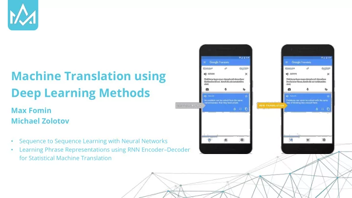
Machine Translation using Deep Learning Methods Max Fomin Michael - PowerPoint PPT Presentation
Machine Translation using Deep Learning Methods Max Fomin Michael Zolotov Sequence to Sequence Learning with Neural Networks Learning Phrase Representations using RNN Encoder Decoder for Statistical Machine Translation Topics
Machine Translation using Deep Learning Methods Max Fomin Michael Zolotov Sequence to Sequence Learning with Neural Networks • Learning Phrase Representations using RNN Encoder – Decoder • for Statistical Machine Translation
Topics Ahead 01 02 03 04 Problem Network Network Results Definition Architecture Training
History of Machine Translation Source Source Source Source Sentence Sentence Sentence Sentence Traditional SMT Traditional SMT Neural Traditional SMT Network Neural Network Neural Network Target Target Target Target Sentence Sentence Sentence Sentence More recently A few years ago Recently
Problem Definition
Types of RNN Problems Regular CNN Image Sentiment Machine Video Model Captioning Analysis Translation Classification
Limitations of current methods Only fixed inputs! Only problems whose inputs and targets can be encoded with fixed dimensionality.
Text Translation! English to French Translation The WMT ’ 14 English to French dataset was used. The models were trained on a subset of 12M sentences consisting of 348M French words and 304M English words. Vocabulary Filtering As typical neural language models rely on a vector representation for each word, we used a fixed vocabulary for both languages. We used 160,000 of the most frequent words for the source language and 80,000 of the most frequent words for the target language. Every out-of-vocabulary word was replaced with a special “ UNK ” token.
The BLEU Score Higher is Better More reference human translations Better and more accurate scores Scores over 30: Understandable translations Scores over 50: Good and fluent translations
Some Background
“ Classical ” RNNs Memory is a powerful tool! Humans don ’ t start their thinking from scratch every second. Sequential Data A recurrent neural network can be thought of as multiple copies of the same network, each passing a message to a successor. This chain-like nature makes them a natural architecture for sequential data.
Long-Term Dependencies “ the clouds are in the sky , ” “ I grew up in France … I speak fluent French . ”
LSTMs Long Short-Term Memory Networks A special kind of RNN, capable of learning long-term dependencies. They work tremendously well on a large variety of problems, and are now widely used. Long-Term Dependencies LSTMs are explicitly designed to avoid the long-term dependency problem. Remembering information for long periods of time is practically their default behavior, not something they struggle to learn!
LSTMs
LSTMs
LSTMs
LSTMs 1 2 3 4
GRUs – Must Be Mentioned! A slightly more dramatic variation on the LSTM It combines the forget and input gates into a single “ update gate. ” It also merges the cell state and hidden state, and makes some other changes. The resulting model is simpler than standard LSTM models, and has been growing increasingly popular.
Network Architecture
High Level Architecture Sequence Input The idea is to use one LSTM to read the input sequence, one time step at a time, to obtain large fixed dimensional vector representation Sequence Output We use another LSTM to extract the output sequence from that vector. The second LSTM is essentially a recurrent neural network language model except that it is conditioned on the input sequence. W X Y Z <EOS> W X Y Z A B C <EOL>
High Level Architecture Overall Process Our method uses a multilayered Long Short-Term Memory (LSTM) to map the input sequence to a vector of a fixed dimensionality, and then another deep LSTM to decode the target sequence from the vector LSTM ENCODER Comment Allez Vous <EOL> How Are You <EOL> LSTM DECODER
A Similar Concept: Word Embeddings
A Similar Concept: Word Embeddings
A Similar Concept: Image Embeddings
A Similar Concept: Multiple Object Embeddings
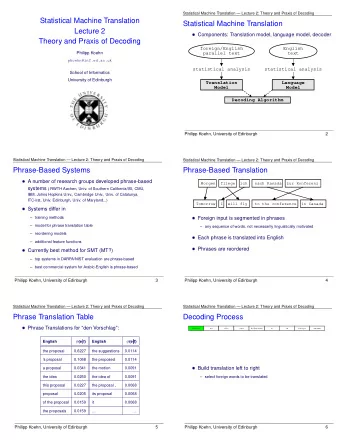
A Classical Approach: Statistical Machine Translation Definition A machine translation paradigm where translations are generated on the basis of statistical models whose parameters are derived from the analysis of bilingual text corpora Goal Finding a translation f, given a source sentence e, which maximizes the 𝑞 𝑔 𝑓 ∝ 𝑞 𝑓 𝑔) 𝑞(𝑔) Phrase Based Creating translation probabilities of matching phrases in the source and target sentences in order to factorize 𝑞 𝑓 𝑔)
Network Training
Classic LSTMs VS Our Model we used two different LSTMs: one for the input sequence and another for the output sequence 𝑞 𝑧 1 , … , 𝑧 𝑈 ′ 𝑦 1 , … , 𝑦 𝑈 = Deep LSTMs significantly outperformed shallow LSTMs, so 𝑈 ′ we chose an LSTM with four layers ෑ 𝑞(𝑧 𝑢 |𝑤, 𝑧 1 , … , 𝑧 𝑢−1 𝑢=1 It was extremely valuable to reverse the order of the words of where, the input sentence 𝑦 1 , … , 𝑦 𝑈 – the input sequence 𝑧 1 , … , 𝑧 𝑈 ′ – the output sequence
Reversed Word Order! LSTM ENCODER <EOL> 𝛿 𝛽 𝛾 C B A <EOL> LSTM DECODER
Training Details 4 layers of LSTMs 1000 cells at each layer 1000 dimensional word embeddings An input vocabulary of 160,000 An output vocabulary of 80,000
Training Details Each additional layer reduced perplexity by nearly 10%. We used a naive softmax over 80,000 words at each output. The resulting LSTM has 380M parameters of which 64M are pure recurrent connections (32M for the “ encoder ” LSTM and 32M for the “ decoder ” LSTM).
Training Details We initialized all of the LSTM ’ s parameters with the uniform distribution between -0.08 and 0.08. We used SGD without momentum, with a fixed learning rate of 0.7. After 5 epochs, we begun halving the learning rate every half epoch. We trained our models for a total of 7.5 epochs. We used batches of 128 sequences for the gradient and divided it the size of the batch. Thus we enforced a hard constraint on the norm of the gradient by scaling it when its norm exceeded a threshold. Different sentences have different lengths. Most sentences are short but some sentences are long. We made sure that all sentences within a mini-batch were roughly of the same length, resulting in a 2x speedup.
Training Details A C++ implementation of deep LSTM with the configuration from the previous section on a single GPU processes a speed of approximately 1,700 words per second. We parallelized our model using an 8-GPU machine. Each layer of the LSTM was executed on a different GPU and communicated its activations to the next GPU (or layer) as soon as they were computed. The remaining 4 GPUs were used to parallelize the softmax, so each GPU was responsible for multiplying by a 1000 × 20000 matrix. The resulting implementation achieved a speed of 6,300 (both English and French) words per second with a minibatch size of 128. Training took about a ten days with this implementation.
Beam-Search Decoder Heuristic Search Algorithm Explores a graph by expanding the most promising node in a limited set. Beam search is an optimization of best-first search that reduces its memory requirements. Greedy Algorithm Best-first search is a graph search which orders all partial solutions (states) according to some heuristic which attempts to predict how close a partial solution is to a complete solution. In beam search, only a predetermined number of best partial solutions are kept as candidates. S A B C D E F G H
Beam-Search Decoder We search for the most likely translation using a simple left-to-right beam search decoder. We maintain a small number B of partial hypotheses. At each time step, we extend each partial hypothesis in the beam with every possible word. we discard all but the B most likely hypotheses according to the model ’ s log probability. As soon as the “ symbol is appended to a hypothesis, it is removed from the beam. A beam of size 2 provides most of the benefits of beam search. S A B C D E F G H
Results
Some Tables
Some Tables
Some Plots
LSTM Hidden States The figure shows a 2D PCA projection of the LSTM hidden states. Notice that both clusters have similar internal structure.
Conclusions A large deep LSTM with a Reversing the words in the limited vocabulary can source sentences gave outperform a standard surprising results SMT-based system with an unlimited vocabulary The ability of the LSTM to A simple straightforward correctly translate very approach can outperform a long sentences was mature SMT system surprising
Thank You!
Recommend
More recommend
Explore More Topics
Stay informed with curated content and fresh updates.
