Machine Learning Prof. Kuan-Ting Lai 2020/4/11 Applied Math for - PowerPoint PPT Presentation
Applied Math for Machine Learning Prof. Kuan-Ting Lai 2020/4/11 Applied Math for Machine Learning Linear Algebra Probability Calculus Optimization Linear Algebra Scalar real numbers Vector (1D) Has a magnitude
Applied Math for Machine Learning Prof. Kuan-Ting Lai 2020/4/11
Applied Math for Machine Learning • Linear Algebra • Probability • Calculus • Optimization
Linear Algebra • Scalar − real numbers • Vector (1D) − Has a magnitude & a direction • Matrix (2D) − An array of numbers arranges in rows & columns • Tensor (>=3D) − Multi-dimensional arrays of numbers
Real-world examples of Data Tensors • Timeseries Data – 3D (samples, timesteps, features) • Images – 4D (samples, height, width, channels) • Video – 5D (samples, frames, height, width, channels) 4
Vector Dimension vs. Tensor Dimension • The number of data in a vector is also called “dimension” • In deep learning , the dimension of Tensor is also called “rank” • Matrix = 2d array = 2d tensor = rank 2 tensor https://deeplizard.com/learn/video/AiyK0idr4uM
The Matrix
Matrix • Define a matrix with m rows and n columns: Santanu Pattanayak , ”Pro Deep Learning with TensorFlow,” Apress, 2017
Matrix Operations • Addition and Subtraction
Matrix Multiplication • Two matrices A and B, where • The columns of A must be equal to the rows of B, i.e. n == p q n • A * B = C, where q • p m m
Example of Matrix Multiplication (3-1) https://www.mathsisfun.com/algebra/matrix-multiplying.html
Example of Matrix Multiplication (3-2) https://www.mathsisfun.com/algebra/matrix-multiplying.html
Example of Matrix Multiplication (3-3) https://www.mathsisfun.com/algebra/matrix-multiplying.html
Matrix Transpose https://en.wikipedia.org/wiki/Transpose
Dot Product • Dot product of two vectors become a scalar • Inner product is a generalization of the dot product • Notation: 𝑤 1 ∙ 𝑤 2 or 𝑤 1𝑈 𝑤 2
Dot Product of Matrix
Linear Independence • A vector is linearly dependent on other vectors if it can be expressed as the linear combination of other vectors • A set of vectors 𝑤 1 , 𝑤 2 , ⋯ , 𝑤 𝑜 is linearly independent if 𝑏 1 𝑤 1 + 𝑏 2 𝑤 2 + ⋯ + 𝑏 𝑜 𝑤 𝑜 = 0 implies all 𝑏 𝑗 = 0, ∀𝑗 ∈ {1,2, ⋯ 𝑜}
Span the Vector Space • n linearly independent vectors can span n -dimensional space
Rank of a Matrix • Rank is: − The number of linearly independent row or column vectors − The dimension of the vector space generated by its columns • Row rank = Column rank • Example: Row- echelon form https://en.wikipedia.org/wiki/Rank_(linear_algebra)
Identity Matrix I • Any vector or matrix multiplied by I remains unchanged • For a matrix 𝐵 , 𝐵𝐽 = 𝐽𝐵 = 𝐵
Inverse of a Matrix • The product of a square matrix 𝐵 and its inverse matrix 𝐵 −1 produces the identity matrix 𝐽 • 𝐵𝐵 −1 = 𝐵 −1 𝐵 = 𝐽 • Inverse matrix is square, but not all square matrices has inverses
Pseudo Inverse • Non-square matrix and have left-inverse or right-inverse matrix • Example: 𝐵𝑦 = 𝑐, 𝐵 ∈ ℝ 𝑛×𝑜 , 𝑐 ∈ ℝ 𝑜 − Create a square matrix 𝐵 𝑈 𝐵 𝐵 𝑈 𝐵𝑦 = 𝐵 𝑈 𝑐 − Multiplied both sides by inverse matrix (𝐵 𝑈 𝐵) −1 𝑦 = (𝐵 𝑈 𝐵) −1 𝐵 𝑈 𝑐 − (𝐵 𝑈 𝐵) −1 𝐵 𝑈 is the pseudo inverse function
Norm • Norm is a measure of a vector’s magnitude • 𝑚 2 norm • 𝑚 1 norm • 𝑚 𝑞 norm • 𝑚 ∞ norm
Eigen Vectors • Eigenvector is a non-zero vector that changed by only a scalar factor λ when linear transform 𝐵 is applied to: 𝐵𝑦 = 𝜇𝑦, 𝐵 ∈ ℝ 𝑜×𝑜 , 𝑦 ∈ ℝ 𝑜 • 𝑦 are Eigenvectors and 𝜇 are Eigenvalues • One of the most important concepts in machine learning, ex: − Principle Component Analysis (PCA) − Eigenvector centrality − PageRank − …
Example: Shear Mapping • Horizontal axis is the Eigenvector
Principle Component Analysis (PCA) • Eigenvector of Covariance Matrix https://en.wikipedia.org/wiki/Principal_component_analysis
NumPy for Linear Algebra • NumPy is the fundamental package for scientific computing with Python. It contains among other things: − a powerful N-dimensional array object − sophisticated (broadcasting) functions − tools for integrating C/C++ and Fortran code − useful linear algebra, Fourier transform, and random number capabilities
Create Tensors Scalars (0D tensors) Vectors (1D tensors) Matrices (2D tensors)
Create 3D Tensor
Attributes of a Numpy Tensor • Number of axes (dimensions, rank) − x.ndim • Shape − This is a tuple of integers showing how many data the tensor has along each axis • Data type − uint8, float32 or float64
Numpy Multiplication
Unfolding the Manifold • Tensor operations are complex geometric transformation in high- dimensional space − Dimension reduction
Basics of Probability
Three Axioms of Probability 𝑂 • Given an Event 𝐹 in a sample space 𝑇, S =ڂ 𝑗=1 𝐹 𝑗 • First axiom − 𝑄 𝐹 ∈ ℝ, 0 ≤ 𝑄(𝐹) ≤ 1 • Second axiom − 𝑄 𝑇 = 1 • Third axiom − Additivity, any countable sequence of mutually exclusive events 𝐹 𝑗 − 𝑄ڂ 𝑗=1 𝑜 𝑜 𝐹 𝑗 = 𝑄 𝐹 1 + 𝑄 𝐹 2 + ⋯ + 𝑄 𝐹 𝑜 = σ 𝑗=1 𝑄 𝐹 𝑗
Union, Intersection, and Conditional Probability • 𝑄 𝐵 ∪ 𝐶 = 𝑄 𝐵 + 𝑄 𝐶 − 𝑄 𝐵 ∩ 𝐶 • 𝑄 𝐵 ∩ 𝐶 is simplified as 𝑄 𝐵𝐶 • Conditional Probability 𝑄 𝐵|𝐶 , the probability of event A given B has occurred 𝐵𝐶 − 𝑄 𝐵|𝐶 = 𝑄 𝐶 − 𝑄 𝐵𝐶 = 𝑄 𝐵|𝐶 𝑄 𝐶 = 𝑄 𝐶|𝐵 𝑄(𝐵)
Chain Rule of Probability • The joint probability can be expressed as chain rule
Mutually Exclusive • 𝑄 𝐵𝐶 = 0 • 𝑄 𝐵 ∪ 𝐶 = 𝑄 𝐵 + 𝑄 𝐶
Independence of Events • Two events A and B are said to be independent if the probability of their intersection is equal to the product of their individual probabilities − 𝑄 𝐵𝐶 = 𝑄 𝐵 𝑄 𝐶 − 𝑄 𝐵|𝐶 = 𝑄 𝐵
Bayes Rule 𝑄 𝐵|𝐶 = 𝑄 𝐶|𝐵 𝑄(𝐵) 𝑄(𝐶) Proof: 𝐵𝐶 Remember 𝑄 𝐵|𝐶 = 𝑄 𝐶 So 𝑄 𝐵𝐶 = 𝑄 𝐵|𝐶 𝑄 𝐶 = 𝑄 𝐶|𝐵 𝑄(𝐵) Then Bayes 𝑄 𝐵|𝐶 = 𝑄 𝐶|𝐵 𝑄(𝐵)/𝑄 𝐶
Naïve Bayes Classifier
Naïve = Assume All Features Independent
Normal (Gaussian) Distribution • One of the most important distributions • Central limit theorem − Averages of samples of observations of random variables independently drawn from independent distributions converge to the normal distribution
Differentiation OR
𝑒𝑧 Derivatives of Basic Function 𝑒𝑦
Gradient of a Function • Gradient is a multi-variable generalization of the derivative • Apply partial derivatives • Example
Chain Rule 46
Maxima and Minima for Univariate Function 𝑒𝑔(𝑦) • If = 0 , it’s a minima or a maxima point, then we study the 𝑒𝑦 second derivative: 𝑒 2 𝑔(𝑦) − If < 0 => Maxima 𝑒𝑦 2 𝑒 2 𝑔(𝑦) − If > 0 => Minima 𝑒𝑦 2 𝑒 2 𝑔(𝑦) − If = 0 => Point of reflection 𝑒𝑦 2 Minima
Gradient Descent
Gradient Descent along a 2D Surface
Avoid Local Minimum using Momentum
Optimization https://en.wikipedia.org/wiki/Optimization_problem
Principle Component Analysis (PCA) • Assumptions − Linearity − Mean and Variance are sufficient statistics − The principal components are orthogonal
Principle Component Analysis (PCA) max. cov 𝐙, 𝐙 𝐗 T 𝐗 = 𝐉 𝑡. 𝑐. 𝑢
References • Francois Chollet , “Deep Learning with Python,” Chapter 2 “Mathematical Building Blocks of Neural Networks” • Santanu Pattanayak , ”Pro Deep Learning with TensorFlow,” Apress, 2017 • Machine Learning Cheat Sheet • https://machinelearningmastery.com/difference-between-a-batch-and-an-epoch/ • https://www.quora.com/What-is-the-difference-between-L1-and-L2-regularization- How-does-it-solve-the-problem-of-overfitting-Which-regularizer-to-use-and-when • Wikipedia
Recommend
More recommend
Explore More Topics
Stay informed with curated content and fresh updates.


