
Machine Learning for Ranking CE-324: Modern Information Retrieval - PowerPoint PPT Presentation
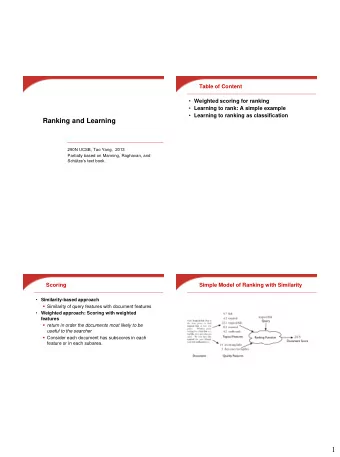
Machine Learning for Ranking CE-324: Modern Information Retrieval Sharif University of Technology M. Soleymani Fall 2015 Some slides have been adapted from: Profs. Manning, Nayak & Raghavan (CS-276, Stanford) Machine learning for IR
Machine Learning for Ranking CE-324: Modern Information Retrieval Sharif University of Technology M. Soleymani Fall 2015 Some slides have been adapted from: Profs. Manning, Nayak & Raghavan (CS-276, Stanford)
Machine learning for IR ranking? We ’ ve looked at methods for ranking docs in IR Cosine similarity, idf, proximity, pivoted doc length normalization, doc autorithy, … We ’ ve looked at methods for classifying docs using supervised machine learning classifiers Naïve Bayes, Rocchio, kNN Surely we can also use machine learning to rank the docs displayed in search results? Sounds like a good idea A.k.a. “ machine-learned relevance ” or “ learning to rank ” 2
Machine learning for IR ranking Actively researched – and actively deployed by major web search engines In the last decade Why didn ’ t it happen earlier? Modern supervised ML has been around for about 20 years … Naïve Bayes has been around for about 50 years … 3
Machine learning for IR ranking The IR community wasn ’ t very connected to the ML community But there were a whole bunch of precursors: Wong, S.K. et al. 1988. Linear structure in information retrieval. SIGIR 1988. Fuhr, N. 1992. Probabilistic methods in information retrieval. Computer Journal. Gey, F. C. 1994. Inferring probability of relevance using the method of logistic regression. SIGIR 1994. Herbrich, R. et al. 2000. Large Margin Rank Boundaries for Ordinal Regression.Advances in Large Margin Classifiers. 4
Why weren ’ t early attempts very successful/influential? Sometimes an idea just takes time to be appreciated … Limited training data Especially for real world use (as opposed to writing academic papers), it was very hard to gather test collection queries and relevance judgments This has changed, both in academia and industry Poor machine learning techniques Insufficient customization to IR problem Not enough features for ML to show value 5
Why wasn ’ t ML much needed? Traditional ranking functions in IR used a very small number of features, e.g., T erm frequency Inverse document frequency Doc length It was easy to tune weighting coefficients by hand And people did 6
Why is ML needed now? Modern systems – especially on the Web – use a great number of features: Arbitrary useful features – not a single unified model Log frequency of query word in anchor text? Query word in color on page? # of images on page? # of (out) links on page? PageRank of page? URL length? URL contains “ ~ ” ? Page edit recency? Page length? The New York Times (2008-06-03) quoted Amit Singhal as saying Google was using over 200 such features. 7
Weighted zone scoring Simple example: Only two zone: title, body 𝑡𝑑𝑝𝑠𝑓 𝑒, 𝑟 = 𝛽𝑇 𝑈 𝑒, 𝑟 + 1 − 𝛽 𝑇 𝐶 𝑒, 𝑟 0 ≤ 𝛽 ≤ 1 We intend to find an optimal value for 𝛽 8
Weighted zone scoring Training examples : each example is a tuple consisting of a query 𝑟 and a doc 𝑒 , together with a relevance judgment 𝑠 for 𝑒 on 𝑟 . In the simplest form, each relevance judgments is either Relevant or Non-relevant . 𝛽 is “ learned ” from examples, in order that the learned scores approximate the relevance judgments in the training examples. 9
Weighted zone scoring 𝑒 1 , 𝑟 1 , 𝑠 (1) , … , 𝑒 𝑂 , 𝑟 𝑂 , 𝑠 (𝑂) 𝐸 = Find minimum of the following cost function: 𝑂 2 𝑠 𝑗 − 𝛽𝑇 𝑈 𝑒 𝑗 , 𝑟 𝑗 − 1 − 𝛽 𝑇 𝐶 𝑒 𝑗 , 𝑟 𝑗 𝐾 𝐸 (𝛽) = 𝑗=1 𝛽 ∗ = argmin 𝐾 𝐸 (𝛽) 0≤𝛽≤1 10
Weighted zone scoring: special case Boolean match in each zone: 𝑇 𝑈 𝑒, 𝑟 , 𝑇 𝐶 𝑒, 𝑟 ∈ {0,1} Boolean relevance judgment: 𝑠 ∈ {0,1} 𝑜 10𝑠 + 𝑜 01𝑜 𝛽 ∗ = 𝑜 10𝑠 + 𝑜 10𝑜 + 𝑜 01𝑜 + 𝑜 01𝑠 𝑜 10𝑠 : number of training data with 𝑇 𝑈 = 1 , 𝑇 𝐶 = 0 and 𝑠 = 1 𝑜 01𝑜 : number of training data with 𝑇 𝑈 = 0 , 𝑇 𝐶 = 1 and 𝑠 = 0 11
Simple example: Using classification for ad-hoc IR Collect a training corpus of (q, d, r) triples Relevance r is here binary (but may be multiclass 3 – 7) Doc is represented by a feature vector 𝒚 = (𝑦 1 , 𝑦 2 ) 𝑦 1 : cosine similarity 𝑦 2 : minimum query window size (shortest text span including all query words) called 𝜕 Query term proximity is a very important new weighting factor Train a model to predict the class 𝑠 of a doc-query pair 12
Simple example: Using classification for ad hoc IR Training data 13
Simple example: Using classification for ad hoc IR A linear score function is then 𝑇𝑑𝑝𝑠𝑓 𝑒, 𝑟 = 𝑥 1 × CosineScore + 𝑥 2 × 𝜕 + 𝑥 0 And the linear classifier is Decide relevant if 𝑇𝑑𝑝𝑠𝑓(𝑒, 𝑟) > 0 just like when we were doing text classification 14
Simple example: Using classification for ad hoc IR cosine score 0.05 Decision R surface R N R R R R R N N R R R N R N N N N N N 0 2 3 4 5 Term proximity 15
More complex example of using classification for search ranking [Nallapati 2004] We can generalize this to classifier functions over more features We can use methods we have seen previously for learning the linear classifier weights 16
Classifier for information retrieval 𝑒, 𝑟 = 𝑥 1 𝑔 1 𝑒, 𝑟 + ⋯ + 𝑥 𝑒 𝑔 𝑒 (𝑒, 𝑟) + 𝑐 Training: (𝑒, 𝑟) must be negative for nonrelevant docs and positive for relevant docs Testing: decide relevant iff (𝑒, 𝑟) ≥ 0 Features are not word presence features To deal with query words not in your training data? but scores like the summed (log) tf of all query terms Unbalanced data Problem: It can result in trivial always-say-nonrelevant classifiers A solution: undersampling nonrelevant docs during training (just take some at random) 17
An SVM classifier for ranking [Nallapati 2004] Experiments: 4 TREC data sets Comparisons with Lemur, a state-of-the-art open source IR engine (Language Model (LM)-based – see IIR ch. 12) 6 features, all variants of tf, idf, and tf.idf scores 18
An SVM classifier for ranking [Nallapati 2004] Train \Test Disk 3 Disk 4-5 WT10G (web) Disk 3 LM 0.1785 0.2503 0.2666 SVM 0.1728 0.2432 0.2750 Disk 4-5 LM 0.1773 0.2516 0.2656 SVM 0.1646 0.2355 0.2675 At best the results are about equal to LM Actually a little bit below Paper ’ s advertisement: Easy to add more features This is illustrated on a homepage finding task onWT10G: Baseline LM 52% p@10, baseline SVM 58% SVM with URL-depth, and in-link features: 78% p@10 19
Learning to rank Classification probably isn ’ t the right way . Classification : Map to a unordered set of classes Regression : Map to a real value Ordinal regression : Map to an ordered set of classes A fairly obscure sub-branch of statistics, but what we want here Ordinal regression formulation gives extra power: Relations between relevance levels are modeled A number of categories of relevance: These are totally ordered: 𝑑 1 < 𝑑 2 < ⋯ < 𝑑 𝐿 Training data: each doc-query pair represented as a feature vector 𝜒 𝑗 and relevance ranking 𝑑 𝑗 as labels 20
Learning to rank: Approaches Point-wise Predicting class label or relevance score Pair-wise Predicting relative order is closer to the nature of ranking than predicting class label or relevance score. Input is a pair of results for a query, and the class is the relevance ordering relationship between them List-wise Learns a ranking function Models the ranking problem in a straightforward fashion. can overcome the drawback of the above approaches by tackling the ranking problem directly 21
Problem with Pointwise Approach Properties of IR evaluation measures have not been well considered. When number of associated docs varies largely for different queries, domination by those queries with a large number of docs. The position of docs in the ranked list is unimportant. The pointwise loss function may unconsciously emphasize too much those unimportant docs (which are ranked low in the final results). 22
Pairwise ranking Goal: classify instance pairs as correctly ranked or incorrectly ranked This turns an ordinal regression problem back into a binary classification problem Advantage Predicting relative order is closer to the nature of ranking than predicting class label or relevance score. Problem The distribution of doc pair number is more skewed than the distribution of doc number, with respect to different queries. 23
The Limitation of Machine Learning Most work produces linear models of features by weighting different base features This contrasts with most of the clever ideas of traditional IR, which are nonlinear scalings and combinations of basic measurements log term frequency, idf, pivoted length normalization 24
Recommend
More recommend
Explore More Topics
Stay informed with curated content and fresh updates.










![Search Evaluation Tao Yang CS290N Slides partially based on text book [CMS] [MRS] Table of](https://c.sambuz.com/1043742/search-evaluation-s.webp)

