Ma c hine L e a rning with MAT L AB - - Re g re ssion Stanley - PDF document

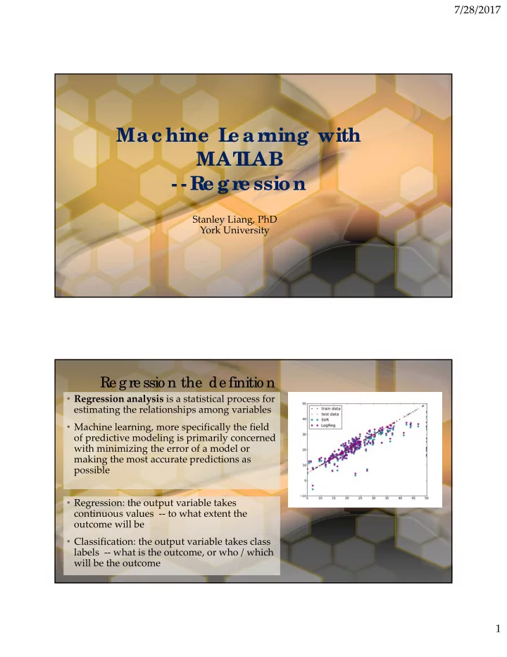
7/28/2017 Ma c hine L e a rning with MAT L AB - - Re g re ssion Stanley Liang, PhD York University Re gre ssio n the de finitio n • Regression analysis is a statistical process for estimating the relationships among variables • Machine learning, more specifically the field of predictive modeling is primarily concerned with minimizing the error of a model or making the most accurate predictions as possible • Regression: the output variable takes continuous values ‐‐ to what extent the outcome will be • Classification: the output variable takes class labels ‐‐ what is the outcome, or who / which will be the outcome 1

7/28/2017 L ine ar Re gre ssio n • Linear regression is developed in the field • When there is a single input variable (x), of statistics and is studied as a model for the method is referred to as simple understanding the relationship between linear regression . When there input and output numerical variables, but are multiple input variables , literature has been borrowed by machine learning. from statistics often refers to the method It is both a statistical algorithm and a as multiple linear regression. machine learning algorithm. • Different techniques can be used to • Linear regression is a linear model , e.g. a prepare or train the linear regression model that assumes a linear relationship equation from data, the most common between the input variables (x) and the of which is called Ordinary Least single output variable (y). More Squares . It is common to therefore refer specifically, that y can be calculated from to a model prepared this way as a linear combination of the input variables Ordinary Least Squares Linear (x). Regression or just Least Squares Regression. • In higher dimensions when we have more than one input (x), the line is called a plane or a hyper ‐ plane. The representation therefore is L ine ar Re gre ssio n the form of the equation and the specific values used for the coefficients • The linear equation assigns one scale factor to each input value or column, called a coefficient • When a coefficient becomes zero, it effectively and represented by the capital Greek letter Beta removes the influence of the input variable on (B). One additional coefficient is also added, the model and therefore from the prediction giving the line an additional degree of freedom made from the model (0 * x = 0). This (e.g. moving up and down on a two ‐ becomes relevant if you look at regularization dimensional plot) and is often called the methods that change the learning algorithm to intercept or the bias coefficient. reduce the complexity of regression models by putting pressure on the absolute size of the coefficients, driving some to zero. 2

7/28/2017 T raining a line ar re gre ssio n mo de l • Learning a linear regression model means estimating the values of the coefficients used in the representation with the data that we have available. • Four techniques to estimate the coefficient (Beta) – Simple Linear Regression: single input – Ordinary Least Squares: >= 2 input – Gradient Descent: most important for ML – Regularization: reduce model complexity and minimize the loss error 1. Lasso Regression: L1 regularization – minimize the absolute sum of coefficients 2. Ridge Regression: L2 regularization – minimize the squared absolute sum of coefficients Pre pare Data fo r L ine ar Re gre ssio n • Linear Assumption: assumes • Gaussian Distributions: Linear that the relationship between your regression will make more reliable input and output is linear ‐‐ need to predictions if your input and output transform data to make the variables have a Gaussian distribution. relationship linear, e.g. exp, log Consider using transforms (e.g. log or BoxCox) on you variables to make • Remove noise: using data cleaning their distribution more Gaussian operations to better expose and looking. clarify the signal in your data, • Rescale Inputs : Linear regression will remove outliers in the output variable (y) if possible often make more reliable predictions if you rescale input variables using • Remove Collinearity: highly standardization or normalization.s correlated input variables will let your model over ‐ fit, compute pairwise correlations of input data and remove the most correlated inputs 3

7/28/2017 Re gre ssio n using SVM and De c isio n T re e s • Parametric regression model • Fit a tree and update it with a SVM regression model • Relation can be specified using a formula – Create a decision tree model by training  easy to interpret data  compute loss (model loss) • Choose a model to generalize all predictor – Use the trained tree model to predict can be difficult – Update the tree model by a SVM model with the polynomial kernel function • If predicting the response for unknown observations is the primary purpose  non ‐ parametric regression – Do not fit the regression model based on a given formula – Can provide more accurate prediction but are difficult to interpret Gaussian Pro c e ss Re gre ssio n • Gaussian process regression (GPR) is a non ‐ parametric regression technique • In addition to predicting the response value for given predictor values, GPR models optionally return the standard deviation and prediction intervals • Fitting Gaussian Process Regression (GPR) Models – mdl = fitrgp(data,responseVarName) • Predicting Response with GPR Models – [yPred,yStd,yInt] = predict(mdl,dataNew) 4

7/28/2017 Re gularize d L ine ar Re gre ssio n • When we have too many predictors, choosing the right type of parametric regression model can be a challenge • A complicated model including all the predictive variables is unnecessary and is likely to become over ‐ fitting • Fitting a linear regression model with a wide table can result in coefficients with large variance • Ridge regression and Lasso help to shrink the regression coefficients Ridge Re gre ssio n • The penalty term – In linear regression, the coefficients are chosen by minimizing the squared difference between the observed and the predicted response value. – This difference is referred to as mean squared error (MSE) – In ridge regression, a penalty term is added to MSE. This penalty term is controlled by the coefficient values and a tuning parameter λ . – The larger the value of λ , the greater the penalty and, therefore, the more the coefficients are “shrunk” towards zero. • Fitting Ridge Regression Models – b = ridge(y,X,lambda,scaling) 5

7/28/2017 L ASSO Re gre ssio n • Lasso (least absolute shrinkage and • [b,fitInfo] = lasso(X,y, ʹ Lambda ʹ ,lambda) selection operator) is a regularized – b ‐ Lasso coefficients. regression method similar to ridge – fitInfo ‐ A structure containing information regression. about the model. – x ‐ Predictor values, specified as a numeric • The difference between the two matrix. methods is the penalty term. In ridge – y ‐ Response values, specified as a vector. regression an L2 norm of the – ʹ Lambda ʹ ‐ Optional property name for coefficients is used whereas in Lasso regularization parameter. an L1 norm is used. – Lambda ‐ Regularization parameter value. • Elastic net – In ridge regression, the penalty term has an L2 norm and in lasso, the penalty term has an L1 norm. You can create regression models with penalty terms containing the combination of L1 and L2 norms. Ste pwise L ine ar Re gre ssio n • Stepwise linear regression methods (stepwiselm) choose a subset of the predictor variables and their polynomial functions to create a compact model • Note that stepwiselm is used only when the underlying model is linear regression • stepwiseMdl = stepwiselm(data,modelspec) – modelspec ‐ Starting model for the stepwise regression – ʹ Lower ʹ and ʹ Upper‘ ‐ limit the complexity of the model – mdl = stepwiselm(data, ʹ linear ʹ , ʹ Lower ʹ , ʹ linear ʹ , ʹ Upper ʹ , ʹ quadratic ʹ ) 6