m-Mode Analysis Imaging with the Owens Valley LWA Michael Eastwood - PowerPoint PPT Presentation
m-Mode Analysis Imaging with the Owens Valley LWA Michael Eastwood California Institute of Technology CALIM2016 October 10, 2016 M. Eastwood m-Mode Analysis Imaging 1 / 24 Caltech Harvard/SAO Gregg Hallinan Lincoln Greenhill
m-Mode Analysis Imaging with the Owens Valley LWA Michael Eastwood California Institute of Technology CALIM2016 – October 10, 2016 M. Eastwood – m-Mode Analysis Imaging 1 / 24 �
Caltech Harvard/SAO Gregg Hallinan Lincoln Greenhill Sandy Weinreb Jonathon Kocz → JPL Stephen Bourke → Chalmers Ben Barsdell → NVIDIA Jake Hartman → Google Danny Price → Berkeley Harish Vedantham Hugh Garsden Kate Clark JPL Marin Anderson Larry D’Addario Ryan Monroe Joe Lazio David Wang and the rest of the LWA team OVRO Dave Woody James Lamb OVRO staff M. Eastwood – m-Mode Analysis Imaging 2 / 24 �
Introduction Foregrounds in 21 cm Cosmology M. Eastwood – m-Mode Analysis Imaging 3 / 24 �
Introduction Foreground Leakage is a Problem z ∼ 8 . 4 Ali et al. (2015) M. Eastwood – m-Mode Analysis Imaging 4 / 24 �
Introduction The 408 MHz Haslam Map Our understanding of the VHF sky is an extrapolation of this map. Haslam et al. (1981, 1982) M. Eastwood – m-Mode Analysis Imaging 5 / 24 �
The Owens Valley LWA The Owens Valley LWA (OVRO LWA) • Dark ages and the cosmic dawn • Radio transients • Extra-solar space weather • Monitoring of the Sun and Jupiter • Ionospheric studies M. Eastwood – m-Mode Analysis Imaging 6 / 24 �
The Owens Valley LWA OVRO LWA Details • 288 crossed-dipole antennas (expanding to 352) • 1.5 km maximum baseline (expanding to 2.5 km) • 512-input LEDA correlator • 24.7 MHz to 82.3 MHz instantaneous • 5 antennas have noise-switched front ends M. Eastwood – m-Mode Analysis Imaging 7 / 24 �
The Owens Valley LWA OVRO LWA Data Reduction Pipeline M. Eastwood – m-Mode Analysis Imaging 8 / 24 �
The Owens Valley LWA TTCal Details • Calibration routine developed for the OVRO LWA • Standard tool for OVRO LWA data reduction • Gain calibration • Polarization calibration • Direction-dependent calibration • Point sources, Gaussians, shapelets, disks, near-field sources • Open source license (GPLv3+) • https://github.com/mweastwood/TTCal.jl M. Eastwood – m-Mode Analysis Imaging 9 / 24 �
The Owens Valley LWA WSClean Snapshot Image OVRO LWA snapshot image provided courtesy of Marin Anderson M. Eastwood – m-Mode Analysis Imaging 10 / 24 �
The Owens Valley LWA BPJSpec Details • m-mode analysis implementation • All-sky images • Foreground filtering • Power spectrum estimation • Open source license (GPLv3+) • https://github.com/mweastwood/BPJSpec.jl M. Eastwood – m-Mode Analysis Imaging 11 / 24 �
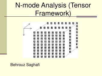
m-Mode Analysis Introduction to m-Mode Analysis A new analysis framework for CHIME-like telescopes. M. Eastwood – m-Mode Analysis Imaging 12 / 24 �
m-Mode Analysis m-Mode Analysis Fundamentals � visibility = (sky brightness) × (beam) × (fringe pattern) dΩ For a telescope that does not steer its beam, visibilities are a periodic function of the sidereal time. visibility sidereal time Fourier transform − − − − − − − − − − − − − − − − − − − − − − → m-mode . . ... . . . . m-modes = transfer matrix a lm . . ... . . . . Shaw et al. (2014, 2015) M. Eastwood – m-Mode Analysis Imaging 13 / 24 �
m-Mode Analysis The Fundamental Equation v = B B Ba + noise v is the vector of m-modes. This is what is measured by the interferometer. B is the transfer matrix. It describes the response of the B B interferometer to the sky. This matrix is block diagonal . a is the vector of spherical harmonic coefficients (for the sky brightness). Shaw et al. (2014, 2015) M. Eastwood – m-Mode Analysis Imaging 14 / 24 �
m-Mode Analysis m-Mode Analysis Imaging Goal: Estimate a given the observations v Least squares minimization a = argmin � v − Ba � 2 = ( B B ) − 1 B B ∗ B B ∗ v ˆ B B B Problem: B B B ∗ B B B is singular! M. Eastwood – m-Mode Analysis Imaging 15 / 24 �
m-Mode Analysis Regularizing the Problem Goal: Estimate a given the observations v , but unmeasured modes should be set to zero. Least squares with Tikhonov regularization � v − Ba � 2 + λ � a � 2 � I ) − 1 B � a = argmin ˆ = ( B B B ∗ B B + λI B I B B ∗ v Problem: How do we choose λ ? (come talk to me!) M. Eastwood – m-Mode Analysis Imaging 16 / 24 �
m-Mode Analysis Advantages of m-Mode Analysis • Exactly incorporates wide-field effects • Automatic deconvolution of large-scales • Uses spherical harmonic basis functions instead of pixels • Uses standard matrix algebra (BLAS, LAPACK) • Block diagonal → big computational savings (over a naive linear algebra approach) M. Eastwood – m-Mode Analysis Imaging 17 / 24 �
m-Mode Analysis Disadvantages of m-Mode Analysis • Only applicable to telescopes that do not steer their beam • Requires data from a full sidereal day • Requires explicit computation of the transfer matrix • The transfer matrix can be very large M. Eastwood – m-Mode Analysis Imaging 18 / 24 �
m-Mode Analysis m-Mode Analysis at the OVRO LWA • Transfer matrix = 500 GB per frequency channel • Computations distributed across 160 workers • 100 hours of integration time • 10 arcminute resolution in the output maps ( l ≤ 1000 ) • 8 maps evenly spaced between 36.528 MHz and 72.152 MHz (each 24 kHz bandwidth) M. Eastwood – m-Mode Analysis Imaging 19 / 24 �
m-Mode Analysis m-Mode Analysis Map at 41.760 MHz CAUTION – very preliminary Eastwood et al. (in prep.) M. Eastwood – m-Mode Analysis Imaging 20 / 24 �
m-Mode Analysis m-Mode Analysis Map at 57.456 MHz CAUTION – very preliminary Eastwood et al. (in prep.) M. Eastwood – m-Mode Analysis Imaging 21 / 24 �
m-Mode Analysis m-Mode Analysis Map at 73.152 MHz CAUTION – very preliminary Eastwood et al. (in prep.) M. Eastwood – m-Mode Analysis Imaging 22 / 24 �
m-Mode Analysis Combined m-Mode Analysis Map CAUTION – very preliminary Eastwood et al. (in prep.) M. Eastwood – m-Mode Analysis Imaging 23 / 24 �
m-Mode Analysis Summary • First demonstration of m-mode analysis imaging • (Preliminary) maps with 10 arcminute resolution • 8 maps evenly spaced between 36.528 MHz and 72.152 MHz (each 24 kHz bandwidth) Come talk to me about: • 21 cm cosmology • Foregrounds in 21 cm cosmology • m-mode analysis • Calibration, source removal, and peeling M. Eastwood – m-Mode Analysis Imaging 24 / 24 �
Backup Slides M. Eastwood – m-Mode Analysis Imaging 25 / 34 �
M. Eastwood – m-Mode Analysis Imaging 26 / 34 �
M. Eastwood – m-Mode Analysis Imaging 27 / 34 �
m-Mode Analysis Scale Map of the Universe Last Scattering Surface 14000 Mpc 14 Gyr M. Eastwood – m-Mode Analysis Imaging 28 / 34 �
m-Mode Analysis Scale Map of the Universe 2dF M. Eastwood – m-Mode Analysis Imaging 28 / 34 �
m-Mode Analysis Scale Map of the Universe Hubble Ultra Deep Field M. Eastwood – m-Mode Analysis Imaging 28 / 34 �
m-Mode Analysis Scale Map of the Universe LWA PAPER CHIME M. Eastwood – m-Mode Analysis Imaging 28 / 34 �
m-Mode Analysis Hyperfine Structure • Proton and electron spins symmetric or antisymmetric • Magnetic dipole transition → very weak • Optically thin tracer of HI M. Eastwood – m-Mode Analysis Imaging 29 / 34 �
m-Mode Analysis Radiative Transfer � T spin − T CMB ( z ) � ∆ T B ∼ 27 x HI (1 + δ ) mK T spin Pritchard & Loeb (2012) M. Eastwood – m-Mode Analysis Imaging 30 / 34 �
m-Mode Analysis Cooling M. Eastwood – m-Mode Analysis Imaging 31 / 34 �
m-Mode Analysis Temperature History M. Eastwood – m-Mode Analysis Imaging 32 / 34 �
m-Mode Analysis Temperature History M. Eastwood – m-Mode Analysis Imaging 32 / 34 �
m-Mode Analysis Temperature History M. Eastwood – m-Mode Analysis Imaging 32 / 34 �
m-Mode Analysis The 21 cm Signal M. Eastwood – m-Mode Analysis Imaging 33 / 34 �
m-Mode Analysis Picking the Regularization Parameter M. Eastwood – m-Mode Analysis Imaging 34 / 34 �
m-Mode Analysis Picking the Regularization Parameter M. Eastwood – m-Mode Analysis Imaging 34 / 34 �
Recommend


More recommend
Explore More Topics
Stay informed with curated content and fresh updates.