LSI system Input v v1 x v1 x v2 x v2 x + + L + v3 x + v3 - PDF document

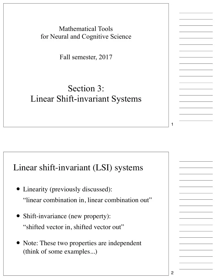
Mathematical Tools for Neural and Cognitive Science Fall semester, 2017 Section 3: Linear Shift-invariant Systems 1 Linear shift-invariant (LSI) systems • Linearity (previously discussed): “linear combination in, linear combination out” • Shift-invariance (new property): “shifted vector in, shifted vector out” • Note: These two properties are independent (think of some examples...) 2

LSI system Input v v1 x v1 x v2 x v2 x + + L + v3 x + v3 x v4 x + v4 x + Output As before, express input as a sum of “impulses”, weighted by elements of x 3 LSI system Input v v1 x v1 x v2 x v2 x + + L + v3 x + v3 x v4 x + v4 x + • Linearity => response to x is sum of Output responses to impulses, weighted by elements of x • Shift-invariance => responses to impulses are shifted copies of each other 4

LSI system Input v v1 x v1 x v2 x v2 x + + L + v3 x + v3 x v4 x + v4 x + Output LSI systems are characterized by their “impulse response” 5 Convolution In r 2 r 1 r 0 r 3 r 2 r 1 X y ( n ) = r ( n − k ) x ( k ) + + k X = r ( k ) x ( n − k ) Out k • Sliding dot products • Matrix description • Boundaries: zero-padded, reflected, circular • Examples: impulse, delay, average, difference 6

Feedback LSI system In r 3 r 2 r 1 • Infinite impulse response (IIR) + • Recursive => possibly unstable Out X X y ( n ) = f ( n − k ) x ( k ) + g ( n − k ) y ( k ) k k (In general, we’ll stick to feedforward (FIR) systems) 7 2D convolution • sliding window [figure c/o Castleman] 8

Discrete Sinusoids “frequency” (cycles/vectorLength) 1 cos( ω n ) , ω = 2 π k/N 0 − 1 0 10 20 30 “frequency” (radians/sample) 1 More generally: 0 − 1 “amplitude” 0 10 20 30 “phase” (radians) 9 Shifting Sinusoids A cos( ω n − φ ) = A cos( φ ) cos( ω n ) + A sin( φ ) sin( ω n ) ... via a well-known trigonometric identity: cos( a − b ) = cos( a ) cos( b ) + sin( a ) sin( b ) We’ll also need conversions between polar and rectangular coordinates: y x = A cos( φ ) , y = A sin( φ ) A φ x 2 + y 2 , p φ = tan − 1 ( y/x ) A = x 10

Shifting Sinusoids A cos( ω n − φ ) = A cos( φ ) cos( ω n ) + A sin( φ ) sin( ω n ) two scale factors: fixed cos/sin vectors: 1 0 A sin φ − 1 A 0 10 20 30 φ 1 A cos φ 0 − 1 0 10 20 30 A scaled and shifted sinusoidal vector can be written as a weighted sum of two fixed sinusoidal vectors! 11 Shifting Sinusoids A cos( ω n − φ ) = A cos( φ ) cos( ω n ) + A sin( φ ) sin( ω n ) fixed cos/sin vectors: A = 1.6, φ = 2 π 1/12 A = 1.6, φ = 2 π 0/12 1 0 − 1 1 1 0 10 20 30 0 0 1 − 1 − 1 0 0 0 10 10 20 20 30 30 − 1 0 10 20 30 A scaled and shifted sinusoidal vector can be written as a weighted sum of two fixed sinusoidal vectors! 12

Shifting Sinusoids A cos( ω n − φ ) = A cos( φ ) cos( ω n ) + A sin( φ ) sin( ω n ) fixed cos/sin vectors: A = 1.6, φ = 2 π 4/12 A = 1.6, φ = 2 π 2/12 A = 1.6, φ = 2 π 3/12 A = 1.6, φ = 2 π 6/12 A = 1.6, φ = 2 π 5/12 1 0 − 1 1 1 1 1 1 0 10 20 30 0 0 0 0 0 1 − 1 − 1 − 1 − 1 − 1 0 0 0 0 0 0 10 10 10 10 10 20 20 20 20 20 30 30 30 30 30 − 1 0 10 20 30 A scaled and shifted sinusoidal vector can be written as a weighted sum of two fixed sinusoidal vectors! 13 LSI response to sinusoids x ( n ) = cos( ω n ) (input) 14

LSI response to sinusoids x ( n ) = cos( ω n ) (convolution formula) L 15 LSI response to sinusoids x ( n ) = cos( ω n ) (trig identity) inner product of impulse response with cos/sin, respectively L 16

LSI response to sinusoids x ( n ) = cos( ω n ) L 17 LSI response to sinusoids x ( n ) = cos( ω n ) (convert rectangular to polar coordinates) A sin φ s r ( ω ) R s ( ω ) A φ A cos φ R c ( ω ) c r ( ω ) 18

LSI response to sinusoids x ( n ) = cos( ω n ) (trig identity, in the opposite direction) L “Sinusoid in, sinusoid out” (with modified amplitude/phase) 19 LSI response to sinusoids More generally, if input has amplitude and phase , A x φ x amplitudes multiply phases add L “Sinusoid in, sinusoid out” (with modified amplitude/phase) 20

The Discrete Fourier transform (DFT) • Construct an orthogonal matrix of sin/cos pairs, covering different numbers of cycles • Frequency multiples of radians/sample, (specifically, ) • For , only need the cosine part (thus, cosines, and sines) N/ 2 + 1 N/ 2 − 1 • When we apply this matrix to an input vector, think of output as paired coordinates • Common to plot these pairs as amplitude/phase [all details on board...] 21 k =0 k =1 k =2 k =3 F = 22

The Fourier family signal domain frequency domain we are here Note: the “fast Fourier transform” (FFT) is a computationally efficient implementation of the DFT. Computational cost is Nlog(N) operations, compared to the N 2 operations that would be needed for matrix multiplication. 23 LSI response to sinusoids x ( n ) = cos( ω n ) NOTE: These dot products are just the Fourier transform of the impulse response r(m) ! 24

Fourier & LSI ⇥ L x 25 Fourier & LSI ⇥ L x note: only 3 (of many) frequency components shown 26

Fourier & LSI ⇥ L x note: only 3 (of many) frequency components shown 27 Fourier & LSI Input ⇥ L x v v1 x v1 x v2 x v2 x + + L v3 x + + v3 x v4 x + + v4 x Output LSI systems are characterized by their frequency response , specified by the Fourier Transform of their impulse response 28

Complex exponentials: “bundling” sine and cosine e i θ = cos( θ ) + i sin( θ ) e i ω n = cos( ω n ) + i sin( ω n ) real part: n imaginary part: n 29 Complex exponentials: “bundling” sine and cosine e i ω n L 30

Complex exponentials: “bundling” sine and cosine e i ω n L F.T. of impulse response! 31 Complex exponentials: “bundling” sine and cosine e i ω n L F.T. of impulse response! L Note: implies that complex exponentials are eigenvectors ! 32

The “convolution theorem” convolve with 33 The “convolution theorem” convolve with Fourier Transform Fourier Transform inverse pointwise multiply by 34

The “convolution theorem” L convolve with Fourier Transform Fourier Transform inverse F T F pointwise multiply by F T ~ y = ˜ RF T ~ x ⇒ (diagonal matrix) 35 Recap • Linear system - defined by superposition - characterized by a matrix • Linear Shift-Invariant (LSI) system - defined by superposition and shift-invariance - characterized by a vector (the impulse response) - alternatively, characterized by frequency response (the Fourier Transform of the impulse response), which specifies an amplitude multiplier and a phase shift for each frequency. 36

What do we do with Fourier Transforms? • Represent/analyze periodic signals • Analyze/design LSI systems . In particular, how do you identify the nullspace? 37 Discrete Fourier transform (with complex numbers) ω k = 2 π k where N N − 1 r n = 1 X r k e i ω k n ˜ (inverse) N k =0 k [on board: why minus sign? why 1/N?] 38

Visualizing the (Discrete) Fourier transform • Two conventional choices for frequency axis: - Plot frequencies from k=0 to k=N/2 (in matlab: 1 to N/2-1) - Plot frequencies from k=-N/2 to N/2-1 (in matab: use fftshift) • Typically, plot Amplitude (and possibly Phase, on a separate graph), instead of the cosine/sine (real/imaginary) parts 39 => Example for k=2, N=32 (note indexing and amplitudes): 1 10 10 0 0 0 (real part) − 10 − 10 − 1 0 10 20 30 0 10 20 30 − 10 0 10 k 1 10 10 0 0 0 (imag part) − 10 − 10 − 1 0 10 20 30 0 10 20 30 − 10 0 10 k 40

More examples • constant • sinusoid (see next slide) • impulse • Gaussian - “lowpass” • DoG (difference of 2 Gaussians) - “bandpass” • Gabor (Gaussian windowed sinusoid) - “bandpass” [on board] 41 Retinal ganglion cells (1D) Enroth-Cugell and Robson (1984) 42

Sampling causes “aliasing” Sampling process is linear, but many-to-one (non-invertible) “Aliasing” - one frequency masquerades as another [on board] Given the samples, it is common/natural to assume that they arose from the lowest compatible frequency... 43 Effect of sampling on the Fourier Transform: Sum of shifted copies | X ( ω ) | | X s ( ω ) | 44

Real-world aliasing downsample by 2 “Moiré pattern” 45 Pre-filtering to avoid spectral overlap (“aliasing”) L ( ω ) | X ( ω ) | lowpass filter, L ( ω ) cutoff at π / ∆ | X s ( ω ) | 46

Real-world aliasing downsample by 2 , with pre-filtering 47