Lower Bounds Best-, Average-, and Worst-Case Time Complexity - PDF document

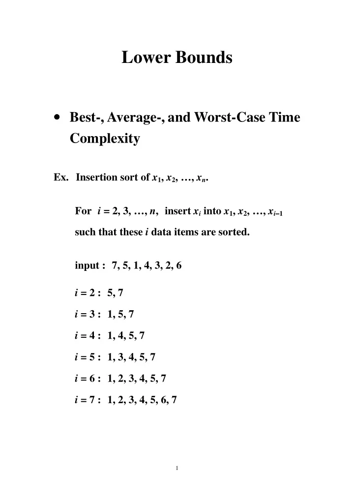
Lower Bounds • • Best-, Average-, and Worst-Case Time • • Complexity Ex. Insertion sort of x 1 , x 2 , …, x n . For i = 2, 3, …, n , insert x i into x 1 , x 2 , …, x i − − 1 − − such that these i data items are sorted. input : 7, 5, 1, 4, 3, 2, 6 i = 2 : 5, 7 i = 3 : 1, 5, 7 i = 4 : 1, 4, 5, 7 i = 5 : 1, 3, 4, 5, 7 i = 6 : 1, 2, 3, 4, 5, 7 i = 7 : 1, 2, 3, 4, 5, 6, 7 1

T ( n ) : the number of comparisons made best case : T ( n ) = O ( n ) worst case : T ( n ) = O ( n 2 ) average case : T ( n ) = O ( n 2 ) Consider the insertion of x i . P ( k ) : the probability of making k comparisons − 2) = 1 ⇒ P (1) = P (2) = … = P ( i − − − i − 1) = 2 P ( i − − − i ⇒ the average number of comparisons for x i × 1 × 2 = (1 + 2 + … + ( i − − 2)) × i + ( i − − 1) × − − × × − − × × i = i + 1 − 1 − − − i 2 The average number of comparisons for n i + 1 1 ∑ = O ( n 2 ). x 2 , x 3 , …, x n is equal to − ( ) i 2 i = 2 2

Ex. Binary search of a 1 , a 2 , …, a n . Assume n = 2 k − − − − 1. T ( n ) : the number of comparisons made best case : T ( n ) = O (1) worst case : T ( n ) = O (log n ) average case : T ( n ) = O (log n ) P ( i ) : the probability of making i comparisons for a successful search i − 1 2 ⇒ P ( i ) = , for i = 1, 2, …, k n The average number of comparisons for a successful search is equal to i − k 1 2 1 ∑ × (2 k ( k − i × × × × × × × − − 1) + 1) = O (log n ). − = n ( ) n i = 1 3

k ∑ i − = 2 k ( k − 1 ( i × × × × − 1) + 1 can be proved by − − 2 ( ) i = 1 induction on k ) There are k = O (log n ) comparisons for each unsuccessful search. Exercise 1. Analyze the time complexity of the quick sort in the best, average, and worst cases. (refer to page 32 of the textbook) 4

• • Lower Bound for a Problem • • A problem has a lower bound of Ω Ω ( g ( n )). Ω Ω ⇒ Any algorithm that can solve it takes ⇒ ⇒ ⇒ Ω ( g ( n )) time. Ω Ω Ω For example, sorting n data items requires Ω ( n log n ) time. Ω Ω Ω Unless stated otherwise, “lower bound” means “lower bound in the worst case”. For a problem, if the time complexity of an algorithm matches a lower bound, then the algorithm is time optimal and the lower bound is tight. Otherwise (if the lower bound is lower than the time complexity of the algorithm), the lower bound or the algorithm can be improved. 5

• • Lower Bound by Comparison Tree • • The method of comparison tree is applicable to comparison-based algorithms which make comparisons among input data items. Most of sorting (exclusive of radix sort and bucket sort), searching, selection, and merging algorithms are comparison-based. The execution of a comparison-based algorithm can be described by a comparison tree, and the tree depth is the greatest number of comparisons, i.e., the worst-case time complexity. ⇒ The minimal tree depth of all possible ⇒ ⇒ ⇒ comparison trees is a lower bound. 6

Ex. Sequential search and binary search of A (1), A (2), …, A ( n ) for x . x A : (1) Failure : (2) x A ... Failure x A n : ( ) Failure Failure   n + 1 x A : ( )     2     n + 1 3 n + 1 : ( ) : ( ) x A   x A       4 4 ... ... ... ...   −   + n + 1 n + 1 x A : (1) x A : (   1) x A : (   1) x A n : ( )     2 2 Failure Failure Failure Failure Failure Failure Failure Failure ⇒ ⇒ Searching has a lower bound of Ω ⇒ ⇒ Ω (log n ). Ω Ω Since binary search takes O (log n ) time, the lower bound is tight. 7

Ex. Sorting a 1 , a 2 , …, a n . Straight insertion sort of a 1 , a 2 , a 3 : Sorting 3, 1, 2 : 3 → → → → 3, 1 → → 1, 3 → → → → → → 1, 3, 2 → → 1, 2, 3 → → ( a 1 : a 2 ) ( a 2 : a 3 ) ( a 1 : a 2 ) Sorting 2, 1, 3 : 2 → → 2, 1 → → → → → → 1, 2 → → → → 1, 2, 3 ( a 1 : a 2 ) ( a 2 : a 3 ) 8

Bubble sort of a 1 , a 2 , a 3 : Sorting 3, 1, 2 : 3, 1, 2 → → → 1, 3, 2 → → → 1, 2, 3 → → ( a 1 : a 2 ) ( a 2 : a 3 ) ( a 1 : a 2 ) Sorting 2, 1, 3 : 2, 1, 3 → → → 1, 2, 3 → ( a 1 : a 2 ) ( a 2 : a 3 ) 9

one-to-one correspondence n ! leaf nodes ← ← ← ←                 →  → → → n ! possible input sequences When the comparison tree is balanced, the tree depth is   log n !   = Ω     Ω ( n log n ) (refer to page 47 of the Ω Ω textbook), which is minimum. Heap sort takes O ( n log n ) time. ⇒ ⇒ Ω ⇒ ⇒ Ω ( n log n ) is tight for sorting. Ω Ω The worst-case time complexity of sorting was considered above. In what follows, the average- case time complexity of sorting is considered. 10

Average time complexity of a sorting algorithm can be estimated as L n !, where L is the total length in the comparison tree from the root to each of the leaf nodes. Let L min be the minimal L of all comparison trees ⇒ L ⇒ ⇒ ⇒ min ! is an average-case lower bound for sorting n L min occurs when the comparison tree is balanced. For example, The left tree has L = 13, and the right tree has L = 12 (= L min for n = 9). 11

Suppose that T is a balanced comparison tree with n ! leaf nodes. Let N = n ! + ( n ! − − − 1) = 2( n !) − − − − − 1. ⇒ ⇒ T is of height h =  ⇒ ⇒    log N    .  Assume that there are x 1 leaf nodes of depth h − − 1 − − and x 2 leaf nodes of depth h . ⇒ ⇒ x 1 + x 2 = n ! ⇒ ⇒ (A) x 1 + 1 2 x 2 = 2 h − − − − 1 ( x 2 is even) (B) (A), (B) ⇒ ⇒ x 1 = 2 h ⇒ ⇒ − 2 h − − 1 ) − − − − − − n !, x 2 = 2( n ! − − − ⇒ ⇒ L min = (2 h ⇒ ⇒ − 2 h − − 1 ) h − − − − − n !)( h − − − − − 1) + 2( n ! − − − − 2 h = ( h + 1) n ! − − − Since log N − − 1 < h ≤ − − ≤ ≤ log N , we have ≤ − 2 log N L min > (log N ) n ! − − − = (log N − − 2) n ! + 1. − − ⇒ L ⇒ ⇒ ⇒ min = Ω Ω ( n log n ) Ω Ω n ! 12

For example, n = 3, N = 11, h = 3, x 1 = 2, and x 2 = 4. ⇒ x 1 + 1 ⇒ ⇒ ⇒ 2 x 2 = 2 2 . Quick sort takes O ( n log n ) time in the average case. ⇒ Ω ⇒ ⇒ ⇒ Ω Ω Ω ( n log n ) is the tight average-case lower bound for sorting. Since the heap sort takes O ( n log n ) time in the worst case, it also takes O ( n log n ) time in the average case. 13

Ex. Selection from n data items. Let L ( n ) denote a lower bound for selecting the greatest data item from a 1 , a 2 , …, a n . Any comparison tree has leaf nodes labeled with a 1 , a 2 , …, a n , and each root-to- a i path represents a process to recognize that a i is the greatest element. Since at least n − − − 1 comparisons are required to − find the greatest data item, each root-to-leaf path has length ≥ ≥ ≥ ≥ n − − − − 1. ⇒ ⇒ L ( n ) = n − ⇒ ⇒ − − 1 − Let L k ( n ) denote a lower bound for Exercise 2. selecting the k greatest data items from a 1 , a 2 , …, a n . Prove that for 2 ≤ ≤ ≤ ≤ k ≤ ≤ ≤ n , ≤ − k +   log n ( n − − k + 2)   .     L k ( n ) ≥ ≥ n − ≥ ≥ − − − − − 1) … ( n − − − (Refer to Section 10.1.3 on page 464 of Ref. (2).) 14

Ex. An n -player tournament. An 8-player tennis tournament. C C H A C E H A B C D E F G H C is the best player. Consider each match a comparison. ⇒ finding the best player is equivalent to finding the greatest data item. According to Exercise 2, finding the first two best − 2 +   log n   matches     players requires at least n − − − There is an approach to finding the first two best − 2 +   log n   matches.     players with exactly n − − − 15

Consider the 8-player tennis tournament again. The best player can be found with 7 (= n − − − 1) − matches. The second best player is one of 3 (=     log n     ) candidates, i.e., D , A , and H . ⇒ The second best player can be found with ⇒ ⇒ ⇒  log n    −     − − − 1 matches. − 2 +    log n    is a tight lower bound   Therefore, n − − − for finding the first two best players. 16

• • Lower Bound by a Particular Problem • • Instance Ex. Merging two sorted sequences a 1 ≤ ≤ ≤ a 2 ≤ ≤ ≤ ≤ ≤ … ≤ ≤ a n and ≤ ≤ b 1 ≤ ≤ b 2 ≤ ≤ … ≤ ≤ b n . ≤ ≤ ≤ ≤ ≤ ≤ Consider a problem instance with a 1 < b 1 < a 2 < b 2 < … < a n < b n . When a 1 < b 1 < a 2 < b 2 < … < a i < b i is obtained, b i +1 must be compared with a i +1 and a i +2 before it is placed properly. ⇒ a lower bound of 2 n − − − − 1 comparisons The merging algorithm, which continuously compares the two currently smallest elements of the two sorted lists and outputs the smaller one, performs 2 n − − − 1 comparisons. − ⇒ the lower bound is tight 17