Lot-by-Lot Acceptance Sampling The Acceptance Sampling Problem A - - PowerPoint PPT Presentation

ST 435/535 Statistical Methods for Quality and Productivity Improvement / Statistical Process Control

Lot-by-Lot Acceptance Sampling

The Acceptance Sampling Problem A company receives a shipment of a product from a supplier. A sample is taken, and each item in the sample is classified as nonconforming or conforming (in acceptance sampling, the language is often “defective” or not). The shipment (or “lot”) is then either accepted or rejected.

1 / 11 Lot-by-Lot Acceptance Sampling The Acceptance Sampling Problem

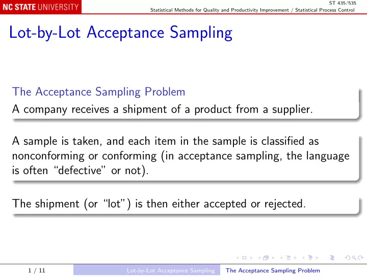
ST 435/535 Statistical Methods for Quality and Productivity Improvement / Statistical Process Control

Important aspects of acceptance sampling: The purpose is to “sentence” lots, not principally to estimate lot quality. Acceptance sampling is not direct quality control. Does not “inspect quality into the product”, just audits output

• f the production process.

Alternatives to acceptance sampling: Accept all lots without inspection; reasonable if supplier’s process capability is high and the process is in statistical control; 100% inspection; when cost of accepting even a single nonconforming item is high.

2 / 11 Lot-by-Lot Acceptance Sampling The Acceptance Sampling Problem

ST 435/535 Statistical Methods for Quality and Productivity Improvement / Statistical Process Control

Single-Sampling Plans for Attributes

Single sample A single random sample of size n is taken from a lot of size N, and each item in the sample is inspected. The lot is found to contain d nonconforming items. The lot is accepted if d ≤ c, the acceptance number, and rejected if d > c. Note that d/n is an unbiased estimate of the lot fraction defective, p.

3 / 11 Lot-by-Lot Acceptance Sampling Single-Sampling Plans for Attributes

ST 435/535 Statistical Methods for Quality and Productivity Improvement / Statistical Process Control

Curtailment Once c + 1 nonconforming items have been found in the sample, we know the lot will be rejected, so inspection could be “curtailed”. But then we know only that d > c, so the unbiased estimate d/n cannot be reported. Consequently, curtailment is not usually recommended in single-sampling plans. However, number nonconforming number inspected is the maximum likelihood estimate of p, even with curtailment.

4 / 11 Lot-by-Lot Acceptance Sampling Single-Sampling Plans for Attributes

ST 435/535 Statistical Methods for Quality and Productivity Improvement / Statistical Process Control

Operating characteristic curve A graph of the probability of accepting a lot versus the lot fraction defective. The random variable D follows the hypergeometric distribution: P(D = d) = k

d

N−k

n−d

• N

n

• ,

max(0, n + k − N) ≤ d ≤ min(n, k) where k = Np is the number of nonconforming items in the lot. Often n ≪ N and the binomial approximation is used: P(D = d) ≈ n d

• pd(1 − p)n−d,

d = 0, 1, . . . , n.

5 / 11 Lot-by-Lot Acceptance Sampling Single-Sampling Plans for Attributes

ST 435/535 Statistical Methods for Quality and Productivity Improvement / Statistical Process Control

In R: Binomial (Type B) OC curves for different sample sizes:

library(AcceptanceSampling); pd <- seq(from = 0, to = 0.08, length = 50); n50c1 <- OC2c(n = 50, c = 1, pd = pd); n100c2 <- OC2c(100, 2, pd = pd); n200c4 <- OC2c(200, 4, pd = pd); plot(n50c1, type = "l"); lines(pd, n100c2@paccept, col = "red"); lines(pd, n200c4@paccept, col = "green"); legend("topright", c("n = 50, c = 1", "n = 100, c = 2", "n = 200, c = 4"), col = c("black", "red", "green"), lty = 1)

6 / 11 Lot-by-Lot Acceptance Sampling Single-Sampling Plans for Attributes

ST 435/535 Statistical Methods for Quality and Productivity Improvement / Statistical Process Control

Effect of changing the acceptance number on the OC curve:

n89c0 <- OC2c(89, 0, pd = pd); n89c1 <- OC2c(89, 1, pd = pd); n89c2 <- OC2c(89, 2, pd = pd); plot(n89c0, type = "l"); lines(pd, n89c1@paccept, col = "red"); lines(pd, n89c2@paccept, col = "green"); legend("topright", c("n = 89, c = 0", "n = 89, c = 1", "n = 89, c = 2"), col = c("black", "red", "green"), lty = 1)

7 / 11 Lot-by-Lot Acceptance Sampling Single-Sampling Plans for Attributes

ST 435/535 Statistical Methods for Quality and Productivity Improvement / Statistical Process Control

By default, OC2c uses the binomial approximation to calculate probabilities (Type B OC curve). Use type = "h" and the N = option to specify a hypergeometric distribution with the given N (Type A OC curve). (But note that pd should be of the form k/N, where k is the number nonconforming in the population.)

plot(OC2c(89, 2, pd = pd, type = "h", N = 500), type = "l")

8 / 11 Lot-by-Lot Acceptance Sampling Single-Sampling Plans for Attributes

ST 435/535 Statistical Methods for Quality and Productivity Improvement / Statistical Process Control

Designing a plan Acceptable quality level (AQL) is poorest quality acceptable as the average. Producer’s risk α is the probability of rejecting a lot with p ≤ AQL. Lot tolerance percent defective (LTPD) is poorest quality acceptable in a single lot. Consumer’s risk β is the probability of accepting a lot with p > LTPD. These four numbers specify two points on the OC curve, and determine n and c.

9 / 11 Lot-by-Lot Acceptance Sampling Single-Sampling Plans for Attributes

ST 435/535 Statistical Methods for Quality and Productivity Improvement / Statistical Process Control

In R: The Producer’s Risk Point (PRP) and Consumer’s Risk Point (CRP) are specified as c(fraction nonconforming, probability of acceptance); for example, c(AQL, 1 − α) and c(LTPD, β):

PRP <- c(0.01, 0.95); CRP <- c(0.06, 0.10); p <- find.plan(PRP = PRP, CRP = CRP, type="binom"); print(p) # n = 110, c = 3

Check the performance:

plot(OC2c(p$n, p$c, pd = pd), type = "l"); points(c(0.01, 0.06), c(0.95, 0.10))

10 / 11 Lot-by-Lot Acceptance Sampling Single-Sampling Plans for Attributes

ST 435/535 Statistical Methods for Quality and Productivity Improvement / Statistical Process Control

A nomograph may also be used to find a plan, as in Section 15.2.3 of the text.

# Montgomery’s suggestion: n89c2 <- OC2c(n = 89, c = 2, pd = pd); assess(n89c2, PRP, CRP); lines(pd, n89c2@paccept, col = "red")

Montgomery’s suggestion requires less inspection, but does not quite meet the Producer Risk Point constraint.

11 / 11 Lot-by-Lot Acceptance Sampling Single-Sampling Plans for Attributes