Logistic Regression (slides borrowed from Tom Mitchell, Barnabs - PowerPoint PPT Presentation

CSCI 4520 - Introduction to Machine Learning Spring 2020 Mehdi Allahyari Georgia Southern University Logistic Regression (slides borrowed from Tom Mitchell, Barnabás Póczos & Aarti Singh 1

Linear Regression & Linear Classification Weight% Height% Linear%decision%boundary% Linear%fit% 2

Naïve Bayes Recap… • NB%Assump$on:% • NB%Classifier:% • Assume%parametric%form%for% P ( X i | Y )%and% P ( Y )% – Es$mate%parameters%using%MLE/MAP%and%plug%in% 3

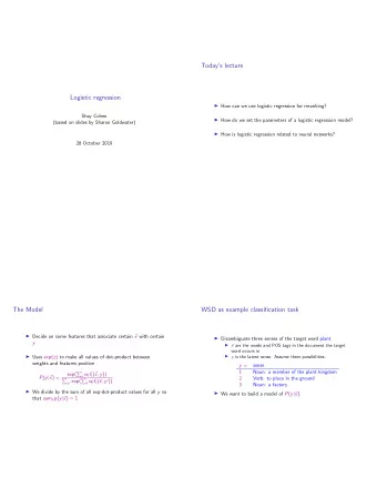
Generative vs. Discriminative Classifiers Genera$ve%classifiers%(e.g.%Naïve%Bayes)% % • %Assume%some%func$onal%form%for%P(X,Y)%(or%P(X|Y)%and%P(Y))% • %Es$mate%parameters%of%P(X|Y),%P(Y)%directly%from%training%data% % But% %arg%max_Y%P(X|Y)%P(Y)%=%arg%max_Y%P(Y|X)% % Why%not%learn%P(Y|X)%directly?%Or%beder%yet,%why%not%learn%the% decision%boundary%directly?% % Discrimina$ve%classifiers%(e.g.%Logis$c%Regression)% % • %Assume%some%func$onal%form%for%P(Y|X)%or%for%the%decision%boundary% • %Es$mate%parameters%of%P(Y|X)%directly%from%training%data% 7% % 4

Logistic Regression Idea: • Naïve Bayes allows computing P(Y|X) by learning P(Y) and P(X|Y) • Why not learn P(Y|X) directly? 5

GNB with equal variance is a linear classifier • Consider learning f: X ! Y, where • X is a vector of real-valued features, < X 1 … X n > • Y is boolean • assume all X i are conditionally independent given Y • model P(X i | Y = y k ) as Gaussian N( µ ik , σ i ) • model P(Y) as Bernoulli ( π ) • What does that imply about the form of P(Y|X)? 6

Derive form for P(Y|X) for Gaussian P(X i | Y=y k ) assuming σ ik = σ i 7

implies implies implies 8

implies implies linear classification rule! implies 9

Logistic Function 10

Logistic regression more generally • Logistic regression when Y not boolean (but still discrete-valued). • Now y ∈ {y 1 ... y R } : learn R-1 sets of weights for k<R for k=R 11

Training Logistic Regression: MCLE We’ll%focus%on%binary%classifica$on:% % • we have L training examples: • maximum likelihood estimate for parameters W • maximum conditional likelihood estimate But there is a problem … Don’t have a model for P(X) or P(X|Y) – only for P(Y|X) 12

Training Logistic Regression: MCLE We’ll%focus%on%binary%classifica$on:% % • we have L training examples: • maximum likelihood estimate for parameters W • maximum conditional likelihood estimate 13

Training Logistic Regression: MCLE • Choose parameters W=<w 0 , ... w n > to maximize conditional likelihood of training data where • Training data D = • Data likelihood = • Data conditional likelihood = 14

Expressing Conditional Log Likelihood 15

Maximizing Conditional Log Likelihood Good news: l ( w ) is a concave function of w → no locally optimal solutions! Bad news: no closed-form solution to maximize l ( w ) Good news: concave functions “easy” to optimize 16

Optimizing concave/convex functions • Condi$onal%likelihood%for%Logis$c%Regression%is%concave% • Maximum%of%a%concave%func$on%=%minimum%of%a%convex%func$on% Gradient(Ascent((concave)/(Gradient(Descent((convex)( Gradient:( Update(rule:( Learning(rate,( η >0( 17

Batch gradient : use error over entire training set D Do until satisfied: 1. Compute the gradient 2. Update the vector of parameters: Stochastic gradient : use error over single examples Do until satisfied: 1. Choose (with replacement) a random training example 2. Compute the gradient just for : 3. Update the vector of parameters: Stochastic approximates Batch arbitrarily closely as Stochastic can be much faster when D is very large Intermediate approach: use error over subsets of D 18

Maximize Conditional Log Likelihood: Gradient Ascent 19

Maximize Conditional Log Likelihood: Gradient Ascent Gradient ascent algorithm: iterate until change < ε For all i , repeat 20

Effect of step size η Large% η %%=>%Fast%convergence%but%larger%residual%error% %%%%%%%%Also%possible%oscilla$ons% % Small% η %%=>%Slow%convergence%but%small%residual%error% %%%% 21

That’s all for M(C)LE. How about MAP? • One common approach is to define priors on W – Normal distribution, zero mean, identity covariance • Helps avoid very large weights and overfitting • MAP estimate • let’s assume Gaussian prior: W ~ N(0, σ ) 22

MLE vs. MAP • Maximum conditional likelihood estimate • Maximum a posteriori estimate with prior W~N(0, σ I ) 23

MAP estimates and Regularization • Maximum a posteriori estimate with prior W~N(0, σ I ) called a “regularization” term • helps reduce overfitting • keep weights nearer to zero (if P(W) is zero mean Gaussian prior), or whatever the prior suggests • used very frequently in Logistic Regression 24

The Bottom Line • Consider learning f: X ! Y, where • X is a vector of real-valued features, < X 1 … X n > • Y is boolean • assume all X i are conditionally independent given Y • model P(X i | Y = y k ) as Gaussian N( µ ik , σ i ) • model P(Y) as Bernoulli ( π ) • Then P(Y|X) is of this form, and we can directly estimate W • Furthermore, same holds if the X i are boolean • trying proving that to yourself 25

Generative vs. Discriminative Classifiers Training classifiers involves estimating f: X ! Y, or P(Y|X) Generative classifiers (e.g., Naïve Bayes) • Assume some functional form for P(X|Y), P(X) • Estimate parameters of P(X|Y), P(X) directly from training data • Use Bayes rule to calculate P(Y|X= x i ) Discriminative classifiers (e.g., Logistic regression) • Assume some functional form for P(Y|X) • Estimate parameters of P(Y|X) directly from training data 26

Use Naïve Bayes or Logistic Regression? Consider • Restrictiveness of modeling assumptions • Rate of convergence (in amount of training data) toward asymptotic hypothesis 27

Use Naïve Bayes or Logistic Regression? Consider Y boolean, X i continuous, X=<X 1 ... X n > Number of parameters to estimate: • NB: • LR: 28

Use Naïve Bayes or Logistic Regression? Consider Y boolean, X i continuous, X=<X 1 ... X n > Number of parameters: • NB: 4n +1 • LR: n+1 Estimation method: • NB parameter estimates are uncoupled • LR parameter estimates are coupled 29

G.Naïve Bayes vs. Logistic Regression Recall two assumptions deriving form of LR from GNBayes: 1. X i conditionally independent of X k given Y 2. P(X i | Y = y k ) = N( µ ik , σ i ), " not N( µ ik , σ ik ) Consider three learning methods: • GNB (assumption 1 only) • GNB2 (assumption 1 and 2) • LR Which method works better if we have infinite training data, and … • Both (1) and (2) are satisfied • Neither (1) nor (2) is satisfied • (1) is satisfied, but not (2) 30

G.Naïve Bayes vs. Logistic Regression G.Naïve Bayes vs. Logistic Regression [Ng & Jordan, 2002] Recall two assumptions deriving form of LR from GNBayes: 1. X i conditionally independent of X k given Y 2. P(X i | Y = y k ) = N( µ ik , σ i ), " not N( µ ik , σ ik ) Consider three learning methods: • GNB (assumption 1 only) -- decision surface can be non-linear • GNB2 (assumption 1 and 2) – decision surface linear • LR -- decision surface linear, trained without assumption 1. Which method works better if we have infinite training data, and... • Both (1) and (2) are satisfied: LR = GNB2 = GNB • (1) is satisfied, but not (2) : GNB > GNB2, GNB > LR, LR > GNB2 • Neither (1) nor (2) is satisfied: GNB>GNB2, LR > GNB2, LR><GNB 31

G.Naïve Bayes vs. Logistic Regression G.Naïve Bayes vs. Logistic Regression [Ng & Jordan, 2002] What if we have only finite training data? They converge at different rates to their asymptotic ( ∞ data) error Let refer to expected error of learning algorithm A after n training examples Let d be the number of features: <X 1 … X d > So, GNB requires n = O(log d) to converge, but LR requires n = O(d) 32

Naïve bayes Logistic Regression Some experiments from UCI data sets [Ng & Jordan, 2002] 33

Naïve Bayes vs. Logistic Regression The bottom line: GNB2 and LR both use linear decision surfaces, GNB need not Given infinite data, LR is better or equal to GNB2 because training procedure does not make assumptions 1 or 2 (though our derivation of the form of P(Y|X) did). But GNB2 converges more quickly to its perhaps-less-accurate asymptotic error And GNB is both more biased (assumption1) and less (no assumption 2) than LR, so either might outperform the other 34

What you should know: • Logistic regression – Functional form follows from Naïve Bayes assumptions • For Gaussian Naïve Bayes assuming variance σ i,k = σ i • For discrete-valued Naïve Bayes too – But training procedure picks parameters without making conditional independence assumption – MLE training: pick W to maximize P(Y | X, W) – MAP training: pick W to maximize P(W | X,Y) • ‘regularization’ • helps reduce overfitting • Gradient ascent/descent – General approach when closed-form solutions unavailable • Generative vs. Discriminative classifiers – Bias vs. variance tradeoff 35