LOGISTIC REGRESSION AND GENERALIZED LINEAR MODELS W. RYAN LEE - PDF document

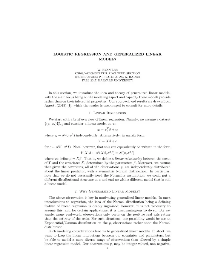
LOGISTIC REGRESSION AND GENERALIZED LINEAR MODELS W. RYAN LEE CS109/AC209/STAT121 ADVANCED SECTION INSTRUCTORS: P. PROTOPAPAS, K. RADER FALL 2017, HARVARD UNIVERSITY In this section, we introduce the idea and theory of generalized linear models, with the main focus being on the modeling aspect and capacity these models provide rather than on their inferential properties. Our approach and results are drawn from Agresti (2015) [1], which the reader is encouraged to consult for more details. 1. Linear Regression We start with a brief overview of linear regression. Namely, we assume a dataset { ( y i , x i ) } n i =1 and consider a linear model on y i : y i = x T i β + ǫ i where ǫ i ∼ N (0 , σ 2 ) independently. Alternatively, in matrix form, Y = Xβ + ǫ for ǫ ∼ N (0 , σ 2 I ). Note, however, that this can equivalently be written in the form Y | X, β ∼ N ( Xβ, σ 2 I ) ≡ N ( µ, σ 2 I ) where we define µ = Xβ . That is, we define a linear relationship between the mean of Y and the covariates X , determined by the parameters β . Moreover, we assume that given the covariates, all of the observations y i are independently distributed about the linear predictor, with a symmetric Normal distribution. In particular, note that we do not necessarily need the Normality assumption; we could put a different distributional structure on ǫ and end up with a different model that is still a linear model. 2. Why Generalized Linear Models? The above observation is key in motivating generalized linear models. In most introductions to regression, the idea of the Normal distribution being a defining feature of linear regression is deeply ingrained; however, it is not necessary to assume this, and for certain applications, it is disadvantageous to do so. For ex- ample, many real-world observations only occur on the positive real axis rather than the entirety of the reals. For such situations, one possibility would be use an Exponential/Gamma distribution on the y i observations rather than the Normal distribution. Such modeling considerations lead us to generalized linear models. In short, we want to keep the linear interactions between our covariates and parameters, but be able to model a more diverse range of observations than allowed by a simple linear regression model. Our observations y i may be integer-valued, non-negative, 1

Generalized Linear Models 2 W. Ryan Lee categorical, or otherwise unsatisfactory for a linear model, but we would still like to be able to model defining characteristics of their distribution (i.e. means, other moments, distributional parameters) using a linear relationship. 3. Natural Exponential Family To delve further into the modeling advantages offered by generalized linear mod- els, we consider the natural exponential family of distributions, of which Normal and Gamma distributions are members. Observations y are said to come from this family if they have a probability density of the form f ( y | θ ) = h ( y ) exp( y T θ − b ( θ )) where θ is called the natural parameter of the distribution. Now consider the log-likelihood, which is the fundamental quantity for statistical inference. l ( θ ) = log f ( y | θ ) Two important identities regarding the log-likelihood concern the expectations of its derivatives, known as the score function S ( θ ) ≡ ∂l ∂θ Note, in particular, that the maximum likelihood estimator is simply the root of the score equation S (ˆ θ ) = 0 Proposition 3.1. Let l ( θ ) be the log-likelihood and S ( θ ) be the score function. Then, under suitable regularity conditions allowing for differentiation under the integral, the following identities hold. � ∂l � E [ S ( θ )] = E = 0 ∂θ � ∂ 2 l � ∂l � 2 � I ( θ ) ≡ − E = E = var ( S ( θ )) ∂θ 2 ∂θ That is, the Fisher information matrix is the variance of the score function. Proof. Letting f ( y | θ ) denote the density, S ( θ ) = ∂ ∂θ log f ( y | θ ) = ∂ θ f ( y | θ ) f ( y | θ ) where ∂ θ denotes the partial derivative with respect to θ , and so the expectation is � ∂ θ f ( y | θ ) � � E [ S ( θ )] = f ( y | θ ) f ( y | θ ) dy = ∂ θ f ( y | θ ) dy = ∂ θ f ( y | θ ) dy = 0 y y y where we use the regularity condition allowing us to take the derivative out of the integral, and note that the integral is always equal to unity by the fact that the integrand is a probability density. For the second identity, note that the first equality is the definition of the Fisher information, and the last identity is true because the expectation of the score is

Generalized Linear Models 3 W. Ryan Lee zero, as we just showed. Thus, the only identity to be proved is the middle identity. We can express the left-hand side as � ∂ 2 l ∂ 2 l � � � ∂θ 2 f ( y | θ ) dy = ∂ θ l ( θ ) ∂ θ f ( y | θ ) | ∞ θ = −∞ − ∂ θ l ( θ ) ∂ θ f ( y | θ ) dy E = ∂θ 2 y y where the second equality follows from integration by parts. The first term is zero for suitable regularity conditions. We now use the expression for the score function to write ∂ θ f ( y | θ ) = ∂ θ l ( θ ) · f ( y | θ ) and so the expression becomes � ∂ 2 l � ∂l � 2 � � ( ∂ θ l ( θ )) 2 f ( y | θ ) dy = E − E = ∂θ 2 ∂θ y as desired. � Using the above proposition, we find the following useful relations regarding the terms in the exponential family density. µ ≡ E [ y | θ ] = b ′ ( θ ) var ( y | θ ) = b ′′ ( θ ) In other words, b ( θ ) is the cumulant function of the distribution. Note in particular that the Poisson, Bernoulli, and Normal distributions are members of the natural exponential family. For example, we can write the proba- bility mass function of a single Poisson observation as f ( y | µ ) = µ y e − µ = ( y !) − 1 exp( y log µ − µ ) y ! which has the form of the exponential family with θ = log( µ ) and b ( θ ) = exp( θ ). Similar derivations can be made for the Bernoulli and Normal cases, among others. An important point to note about exponential family distributions is that they are completely characterized by the relation between the mean and the variance. Theorem 3.2. Let f ( y | θ ) be a density in the natural exponential family. Then, the variance of the distribution can be written in terms of its mean µ ; that is, var ( y | θ ) = v ( µ ) for some function v . Moreover, the function v uniquely specifies the distribution f . For example, the Poisson distributed can be defined as the exponential family distribution such that var( y | µ ) ≡ v ( µ ) = µ and similarly for the Bernoulli and Normal distributions. In other words, there is only one exponential family distribution satisfying the relation v ( µ ) = µ , and this is the Poisson distribution.

Generalized Linear Models 4 W. Ryan Lee 4. Logistic Regression Let us now consider the case of logistic regression to see an example in which the linear model is entirely inadequate. We now assume binary data , in which y take only the values 0 , 1. The model is typically given by logit( µ ) = x T β which implicitly models the observations y as y | µ ∼ Bern( µ ) independently. That is, the observations given the probability µ (or mean) are independently drawn from a Bernoulli distribution, each with its own probability of success µ . These µ are related to the covariates x through a linear predictor of their logit: logit( µ ) ≡ log( µ/ (1 − µ )) Putting this all together, we can write the model as: exp( x T β ) � � = Bern(logit − 1 ( x T β )) y | x, β ∼ Bern 1 + exp( x T β ) where logit − 1 ( x ) = e x / (1 + e x ) is the inverse of the logit function defined above. The logit can be shown to be a reasonable function linking the linear predictor to the mean in a number of ways. When the covariates are also given a distribution and assumed to come from a Normal distribution, then the posterior distribution of y is precisely given by the logistic regression equation above. In addition, when the Bernoulli distribution is written in the exponential family form, one can see that the natural parameter is precisely the logit, as we show below. One interesting property of logistic regression models for classification is implied by their roots in linear models. Often, for classification purposes, one would like to predict the class (0 or 1) of a new sample ˜ y based on a model fit on the existing data. In this case, we would like to predict ˜ y = 1 if x T β ) exp(˜ P (˜ y = 1 | ˜ x, β ) ≡ ˜ µ ≡ x T β ) ≥ c 1 + exp(˜ for some constant c , generally c = 1 / 2. Proposition 4.1. The predictive classification of ˜ x based on the criterion P (˜ y = 1 | ˜ x, β ) ≥ c for any c ∈ (0 , 1) is equivalent to the linear discriminant or linear decision boundary given by x T β ≥ logit ( c ) ˜ Proof. We first prove that the inverse logit is a monotonically increasing function. ∂ x logit − 1 ( x ) = e x (1 + e x ) − e x · e x e x = (1 + e x ) 2 > 0 (1 + e x ) 2 for any finite value of x . Thus, since the inverse logit function is a monotonically increasing function of its argument, it is one-to-one, an inverse exists (the logit), and the inequality logit − 1 ( x ) ≥ c is equivalent to x ≥ logit( c ). �