Local algorithms and max-min linear programs Patrik Floren, Marja - PowerPoint PPT Presentation
Local algorithms and max-min linear programs Patrik Floren, Marja Hassinen, Joel Kaasinen, Petteri Kaski, Topi Musto, Jukka Suomela HIIT, University of Helsinki, Finland TU Braunschweig 11 September 2008 Local algorithms Local
Local algorithms and max-min linear programs Patrik Floréen, Marja Hassinen, Joel Kaasinen, Petteri Kaski, Topi Musto, Jukka Suomela HIIT, University of Helsinki, Finland TU Braunschweig 11 September 2008
Local algorithms Local algorithm: output of a node is a function of input within its constant-radius neighbourhood (Linial 1992; Naor and Stockmeyer 1995) 2 / 39
Local algorithms Local algorithm: changes outside the local horizon of a node do not affect its output (Linial 1992; Naor and Stockmeyer 1995) 3 / 39
Local algorithms Local algorithms are efficient: ◮ Space and time complexity is constant per node ◮ Distributed constant time (even in an infinite network) . . . and fault-tolerant: ◮ Topology change only affects a constant-size part (Naor and Stockmeyer 1995) ◮ Can be turned into self-stabilising algorithms (Awerbuch and Sipser 1988; Awerbuch and Varghese 1991) (In this presentation, we assume bounded-degree graphs) 4 / 39
Local algorithms Applications beyond distributed systems: ◮ Simple linear-time centralised algorithm ◮ In some cases randomised, approximate sublinear-time algorithms (Parnas and Ron 2007) Consequences in theory of computing: ◮ Bounded-fan-in, constant-depth Boolean circuits: in NC 0 ◮ Insight into algorithmic value of information (cf. Papadimitriou and Yannakakis 1991) 5 / 39
Local algorithms Great, but do they exist? Fundamental hurdles: 1. Breaking the symmetry: e.g., colouring a ring of identical nodes 2. Non-local problems: e.g., constructing a spanning tree Strong negative results are known: ◮ 3-colouring of n -cycle not possible, even if unique node identifiers are given (Linial 1992) ◮ No constant-factor approximation of vertex cover, etc. (Kuhn et al. 2004; Kuhn 2005) 6 / 39
Local algorithms Side information Many positive results are known, if we assume some side information (e.g., coordinates, clustering) (Czyzowicz et al. 2008; Floréen et al. 2007; Hassinen et al. 2008; Urrutia 2007; Wang and Li 2006; Wiese and Kranakis 2008; . . . ) Side information helps to break the symmetry But what if we have no side information? 7 / 39
Local algorithms Some previous positive results: ◮ Locally checkable labellings (Naor and Stockmeyer 1995) ◮ Dominating set (Kuhn and Wattenhofer 2005; Lenzen et al. 2008) ◮ Packing and covering LPs (Papadimitriou and Yannakakis 1993; Kuhn et al. 2006) Present work: ◮ Max-min LPs (Floréen et al. 2008a,b,c,d) 8 / 39
Max-min linear program Let A ≥ 0, c k ≥ 0 Objective: maximise min k ∈ K c k · x A x ≤ 1 , subject to x ≥ 0 Generalisation of packing LP: c · x maximise subject to A x ≤ 1 , x ≥ 0 9 / 39
Max-min linear program Let A ≥ 0, C ≥ 0 Equivalent formulation: maximise ω subject to A x ≤ 1 , C x ≥ ω 1 , x ≥ 0 Applications: mixed packing and covering, linear equations find x s.t. A x ≤ 1 , find x s.t. A x = 1 , C x ≥ 1 , x ≥ 0 x ≥ 0 10 / 39
Max-min linear program Distributed setting: ◮ one node v ∈ V for each variable x v , one node i ∈ I for each constraint a i · x ≤ 1, one node k ∈ K for each objective c k · x ◮ v ∈ V and i ∈ I adjacent if a iv > 0, v ∈ V and k ∈ K adjacent if c kv > 0 maximise min k ∈ K c k · x subject to A x ≤ 1 , x ≥ 0 11 / 39
Max-min linear program Distributed setting: ◮ one node v ∈ V for each variable x v , one node i ∈ I for each constraint a i · x ≤ 1, one node k ∈ K for each objective c k · x ◮ v ∈ V and i ∈ I adjacent if a iv > 0, v ∈ V and k ∈ K adjacent if c kv > 0 Key parameters: ◮ ∆ I = max. degree of i ∈ I ◮ ∆ K = max. degree of k ∈ K 12 / 39
Example Task: Data gathering in a sensor network ◮ circle = sensor ◮ square = relay ◮ edge = network connection 13 / 39
Example Task: Maximise the minimum amount of data gathered from each sensor 9 maximise min { 8 x 1 , x 2 + x 4 , 7 x 3 + x 5 + x 7 , 6 x 6 + x 8 , x 9 5 } 4 3 2 1 14 / 39
Example Task: Maximise the minimum amount of data gathered from each sensor; each relay has a limited battery capacity 9 maximise min { 8 x 1 , x 2 + x 4 , 7 x 3 + x 5 + x 7 , 6 x 6 + x 8 , x 9 5 } 4 subject to x 1 + x 2 + x 3 ≤ 1 , 3 x 4 + x 5 + x 6 ≤ 1 , 2 x 7 + x 8 + x 9 ≤ 1 , 1 x 1 , x 2 , . . . , x 9 ≥ 0 15 / 39
Example Task: Maximise the minimum amount of data gathered from each sensor; each relay has a limited battery capacity 9 An optimal solution: 8 x 1 = x 5 = x 9 = 3 / 5 , 7 x 2 = x 8 = 2 / 5 , 6 x 4 = x 6 = 1 / 5 , 5 x 3 = x 7 = 0 4 3 2 1 16 / 39
Example Communication graph: G = ( V ∪ I ∪ K , E ) k ∈ K v ∈ V maximise min { i ∈ I x 1 , x 2 + x 4 , x 3 + x 5 + x 7 , x 6 + x 8 , x 9 } subject to x 1 + x 2 + x 3 ≤ 1 , x 4 + x 5 + x 6 ≤ 1 , x 7 + x 8 + x 9 ≤ 1 , x 1 , x 2 , . . . , x 9 ≥ 0 17 / 39
Example Communication graph: G = ( V ∪ I ∪ K , E ) k ∈ K v ∈ V maximise min { i ∈ I x 1 , x 2 + x 4 , x 3 + x 5 + x 7 , x 6 + x 8 , x 9 } subject to x 1 + x 2 + x 3 ≤ 1 , x 4 + x 5 + x 6 ≤ 1 , x 7 + x 8 + x 9 ≤ 1 , x 1 , x 2 , . . . , x 9 ≥ 0 18 / 39
Example Communication graph: G = ( V ∪ I ∪ K , E ) k ∈ K v ∈ V maximise min { i ∈ I x 1 , x 2 + x 4 , x 3 + x 5 + x 7 , x 6 + x 8 , x 9 } subject to x 1 + x 2 + x 3 ≤ 1 , x 4 + x 5 + x 6 ≤ 1 , x 7 + x 8 + x 9 ≤ 1 , x 1 , x 2 , . . . , x 9 ≥ 0 19 / 39
Old results “Safe algorithm”: Node v chooses 1 x v = min a iv |{ u : a iu > 0 }| i : a iv > 0 (Papadimitriou and Yannakakis 1993) Factor ∆ I approximation Uses information only in radius 1 neighbourhood of v A better approximation ratio with a larger radius? 20 / 39
New results, general case The safe algorithm is factor ∆ I approximation Theorem For any ǫ > 0 , there is a local algorithm for max-min LPs with approximation ratio ∆ I ( 1 − 1 / ∆ K ) + ǫ Theorem There is no local algorithm for max-min LPs with approximation ratio ∆ I ( 1 − 1 / ∆ K ) Degree of a constraint i ∈ I is at most ∆ I Degree of an objective k ∈ K is at most ∆ K 21 / 39
New results, bounded growth Assume bounded relative growth beyond radius R : | B ( v , r + 2 ) | ≤ 1 + δ for all v ∈ V , r ≥ R | B ( v , r ) | where B ( v , r ) = agents in radius r neighbourhood of v Theorem There is a local algorithm for max-min LPs with approximation ratio 1 + 2 δ + o ( δ ) There is no local algorithm for max-min LPs with approximation ratio 1 + δ/ 2 (assuming ∆ I ≥ 3, ∆ K ≥ 3, 0 . 0 < δ < 0 . 1) 22 / 39
Approximability, bounded growth Step 1: Choose local constant-size subproblems Step 3: Solve them optimally Step 3: Take averages of local solutions, add some slack 23 / 39
Approximability, general case Preliminary step 1: Unfold the graph into an infinite tree b a c a c d c a a c b b d c a b b b d d a a c c c d b d c a a b b d d 24 / 39
Approximability, general case Preliminary step 2: Apply a sequence of local transformations (and unfold again) �→ �→ �→ �→ 25 / 39
Approximability, general case It is enough to design a local approximation algorithm for the following special case: ◮ Communication graph G is an (infinite) tree ◮ Degree of each constraint i ∈ I is exactly 2 ◮ Degree of each objective k ∈ K is at least 2 ◮ Each agent v ∈ V adjacent to at least one constraint ◮ Each agent v ∈ V adjacent to exactly one objective ◮ c kv ∈ { 0 , 1 } 26 / 39
Approximability, general case After the local transformations, we have an infinite tree with a fairly regular structure In a centralised setting, we could organise the nodes into layers Then we could design an approximation algorithm. . . 27 / 39
Approximability, general case “Switch off” every R th layer of objectives 28 / 39
Approximability, general case “Switch off” every R th layer of objectives Consider all possible locations (shifting strategy) 29 / 39
Approximability, general case “Switch off” every R th layer of objectives Consider all possible locations (shifting strategy) 30 / 39
Approximability, general case “Switch off” every R th layer of objectives Consider all possible locations (shifting strategy) Solve the LP for the “active” layers, take averages Factor R / ( R − 1 ) approximation 31 / 39
Approximability, general case We could solve the LP simply by propagating information upwards between a pair of “passive” layers But we cannot choose the layers by any local algorithm! Two fundamentally different roles for agents: “up” and “down” How to choose the roles? How to break the symmetry? 32 / 39
Approximability, general case Trick: consider both possible roles for each agent, “up” an “down” Compute locally two candidate solutions, one for each role Take averages Surprise: factor ∆ I ( 1 − 1 / ∆ K ) + ǫ approximation, best possible! 33 / 39
Approximability, general case Some complications: ◮ several optimal solutions ◮ how to make sure that the local choices are “compatible” with each other? Key idea: ◮ “down” nodes choose as large values as possible ◮ “up” nodes choose as small values as possible 34 / 39
Inapproximability Regular high-girth graph or regular tree? 35 / 39
Inapproximability Locally indistinguishable 36 / 39
Recommend


![procedure SERIAL MIN ( A , n ) 1. 2. begin 3. min = A [ 0 ] ; 4. for i := 1 to n 1 do 5.](https://c.sambuz.com/901885/procedure-serial-min-a-n-1-2-begin-3-min-a-0-4-for-i-1-to-s.webp)


More recommend
Explore More Topics
Stay informed with curated content and fresh updates.