Linear programming Input: System of inequalities or equalities over - PowerPoint PPT Presentation
Linear programming Input: System of inequalities or equalities over the reals R A linear cost function Output: Value for variables that minimizes cost function Example: Minimize 6x+4y Subject to 3x + 2y + 5z 1 z = 2 Note:
Linear programming
● Input: System of inequalities or equalities over the reals R A linear cost function ● Output: Value for variables that minimizes cost function Example: Minimize 6x+4y Subject to 3x + 2y + 5z ≥ 1 z = 2 ● Note: Can equivalently maximize the negative of the cost function
● Max flow is a special case of LP Variables: ?
● Max flow is a special case of LP Variables: f(u,v) Max ?
● Max flow is a special case of LP Variables: f(u,v) Max f(s,V) subject to ?
● Max flow is a special case of LP Variables: f(u,v) Max f(s,V) subject to f(v,V)=0 f(u,v) ≤ c(u,v) f(u,v) = -f(v,u)
● Standard form: Min c.x Ax = b x ≥ 0 ● Claim: The general form can be reduced to the standard ● Proof: Express inequality a i . x ≥ b i as a i . x - s i = b i and s i ≥ 0 ∈ + - x - ) with x + ≥ 0, x - ≥ 0 Express x R as (x
● Definition: P := {x : Ax=b, x ≥ 0}, known as polytope ∃ ∈ ∈ x is vertex if not y ≠ 0 : x+y P and x-y P ∈ ● Claim: If min {c.x : x P} is finite, it is achieved at a vertex. ● Proof: ∈ ∈ Suppose x not a vertex. Take y ≠ 0 : x+y P and x-y P. Assume cy < 0, then x+y is a better solution Assume cy > 0, then x-y is a better solution
● Definition: P := {x : Ax=b, x ≥ 0}, known as polytope ∃ ∈ ∈ x is vertex if not y ≠ 0 : x+y P and x-y P ∈ ● Claim: If min {c.x : x P} is finite, it is achieved at a vertex. ● Proof: ∈ ∈ Suppose x not a vertex. Take y ≠ 0 : x+y P and x-y P. Assume cy = 0. Can assume y j < 0 for some j, since y ≠ 0. ∈ Note x + λ y P since Ay = 0 as A(x-y) = A(x+y) = b Increase λ from 0 until one more variable is 0. Note that if a var. was zero it still is, because x i = 0 y i = 0 ∈ ∈ otherwise can't be x+y P and x-y P Have new x' with one more zero variable, and no worse cost Repeat whole argument on x'. This will eventually stop as (0, 0, …, 0) is a vertex.
● This motivates looking for solutions at vertices The simplex algorithm moves from vertex to vertex
● Most basic example of simplex algorithm: min x + y : 2x + 3y=1, x, y ≥ 0. Vertices = (0,1/3), (1/2,0). Somehow start at vertex s 1 := (1/2,0) Write x = 2 -1 ( 1 - 3y) (var > 0 as function of var = 0) Cost = x + y = 2 -1 ( 1 - 3y) + y = 0.5 - 0.5y. Can increment y and reduce the cost, as long as x ≥ 0 This takes us to s 2 := (0,1/3) Write y = 3 -1 (1-2x). Cost = x + y = x + 1/3-2x/3 = x/3 + 1/3. Note this holds for any solution. s 2 has x = 0 so is optimal.
● The simplex method: min c.x : Ax=b, x ≥ 0. Start with some solution s B := {j : s j > 0}, let A B = columns of A corresponding to B N := the other coordinates Assume A B is invertible min c B .x B + c N .x N : A B x B +A N x N = b, x ≥ 0. Write x B = A B -1 (b - A N x N ) Cost = c B A B -1 (b - A N x N ) + c N x N = c B A B -1 b + x N (c N - c B A B -1 A N ) r
● Cost = c B A B -1 b + x N r ● If r j < 0 for some j, increase corresponding var in x N in current solution s as much as possible, to arrive to s'. Now the increased variable is > 0, and another will be 0 s' has smaller cost. Repeat. ● If r ≥ 0, note this holds for every solution. Current solution has x N = 0, so it is optimal. ∈ Note: New solution s is vertex, because if s+y and s-y P then y N is 0; but x B is a function of x N so that stays same too.
Note: We assumed A B is invertible This is not always the case, e.g. if you have too many zero variables. In general, this may make the simplex algorithm take exponential time or even never terminate. There exist more complicated, polynomial-time algorithms However the simplex works well in practice Research in the area is still very active.
● Example: Minimize 6x 1 + 4x 2 Subject to 2x 1 + 3x 2 = 9 x 1 + x 3 = 3 x 1 , x 2 , x 3 ≥ 0 min c.x : Ax=b, x ≥ 0. A = 2 3 0 b = [9 3] T c = [6 4 0] 1 0 1 Start with s = (3, 1, 0)
min c.x : Ax=b, x ≥ 0. A = 2 3 0 b = [9 3] T c = [6 4 0] 1 0 1 Let's start with s = (3, 1, 0) B := {j : s j > 0} = {1, 2} A B = 2 3 A N = 0 A B -1 = 0 1 N := {3} 1 0 1 1/3 -2/3 r = (c N - c B A B -1 A N ) c B = [6 4] c N = [0] = 0 - 10/3 = -10/3 r < 0, so increase x 3 as much as possible, arrive to s' = (0, 3, 3)
min c.x : Ax=b, x ≥ 0. A = 2 3 0 b = [9 3] T c = [6 4 0] 1 0 1 Now we are at s' = (0, 3, 3). Repeat. B := {j : s j > 0} = {2, 3} A B = 3 0 A N = 2 A B -1 = 1/3 0 N := {1} 0 1 1 0 1 r = (c N - c B A B -1 A N ) c B = [4 0] c N = [6] = 6 Since r ≥ 0, s' = (0, 3, 3) is an optimal solution, and the optimal value is 12.
● Duality: z : min x 1 + 2x 2 + 4 x 3 = cx subject to x 1 + x 2 + 2x 3 = 5 2x 1 + x 2 + 3x 3 = 8 x ≥ 0 Want: Best lower bound on z: Can you think of any lower bound?
● Duality: z : min x 1 + 2x 2 + 4 x 3 = cx subject to x 1 + x 2 + 2x 3 = 5 2x 1 + x 2 + 3x 3 = 8 x ≥ 0 Want: Best lower bound on z: 1st equation z ≥ ?
● Duality: z : min x 1 + 2x 2 + 4 x 3 = cx subject to x 1 + x 2 + 2x 3 = 5 2x 1 + x 2 + 3x 3 = 8 x ≥ 0 Want: Best lower bound on z: 1st equation z ≥ 5 A better lower bound?
● Duality: z : min x 1 + 2x 2 + 4 x 3 = cx subject to x 1 + x 2 + 2x 3 = 5 2x 1 + x 2 + 3x 3 = 8 x ≥ 0 Want: Best lower bound on z: 1st equation z ≥ 5 3(1st) - 2nd x 1 + 2x 2 + 3x 3 = 7 ≤ z This process can be automated: Find max 5 y 1 + 8 y 2 subject to y 1 + 2y 2 ≤ 1 (1st column ≤ c 1 ) y 1 + y 2 ≤ 2 (2nd ≤ c 2 ) 2y 1 + 3y 2 ≤ 4 (3rd ≤ c 3 )
● Duality: Consider primal: min cx : Ax=b, x ≥ 0 Suppose we multiply each equation by a number y j and sum: We get y Ax = y b. Now, if yA ≤ c, then yAx ≤ cx, because x ≥ 0 Note yAx = yb. So a generic lower bound is given by dual: max yb : yA ≤ c equivalently, max yb: A T y ≤ c Note: the dual of the dual is the primal.
● Linear programming duality theorem: min cx : Ax=b, x ≥ 0 = max by : A T y ≤ c when they are both finite. A.k.a. min-max theorem, Hahn–Banach theorem
● Main tool in proving duality: Farkas' lemma. ● Recall fundamental theorem of linear algebra ∃ x : Ax = b XOR y such that yA = A ∃ T y = 0 and b.y ≠ 0 i.e., b is in the span of the columns iff b is orthogonal to any vector that is orthogonal to the columns of A ● Farkas lemma: ∃ x : Ax ≤ b XOR y ≥ 0 : yA = A ∃ T y = 0 but b.y = -1 ● Given Farkas' lemma, proof of duality is mostly notation
Duality proof: p* := min {cx : Ax=b, x ≥ 0} d* := max {by: A T y ≤ c } Weak duality: p* ≥ d* Proof: Let c x* = p*, by* = d*, where x* and y* feasible. Then A T y* ≤ c T y* x* ≤ c*x = p*. A But A T y* x* = y* b = d*.
Duality proof: p* := min {cx : Ax=b, x ≥ 0} d* := max {by: A T y ≤ c } Strong duality: p* ≤ d* We want y : A T y ≤ c and b.y ≥ p*. We express this as A T y ≤ c -b -p* ∃ If no such y, by Farkas z ≥ 0 : [A -b] z = 0, [c -p*]z = -1 < 0 Write z = [x, λ ] Ax = λ b, cx < λ p* Case λ > 0. Let x' := x/ λ. Then Ax' = b and cx' < p* Case λ = 0. Then Ax = 0, cx < 0. So A(x+x*) = b, c(x+x*) < p* In either case we contradict the optimality of p*.
∃ ∃ T y = 0 and b.y = -1 Farkas: x : Ax ≤ b XOR y ≥ 0 : yA = A Proof By induction on number of variables Base case: zero variables. The system is of the form 0 ≤ b. ∀ If b i ≥ 0 i then we have a solution but can't get b.y = - 1 Otherwise b i < 0 for some i. In this case there is no solution. Then letting y i = 1/b i and the rest 0 we get b.y = -1.
∃ ∃ T y = 0 and b.y = -1 Farkas: x : Ax ≤ b XOR y ≥ 0 : yA = A Proof Induction step Write x = (x',t). Up to non-negative scaling, each equation in Ax ≤ b is one of: + (x') + t ≤ b i , a i - (x') - t ≤ b i , a i 0 (x') ≤ b i a i For any x', above system solvable in t iff ∀ ∀ 0 (x') ≤ b i - (x') - b i ≤ b j - a j + (x') a i i, and a i, j i If such an x' exists, we have a solution x = (x',t). There is no y ≥ 0 : yA = 0 and b.y = -1, since otherwise, as seen before, from Ax ≤ b we obtain that 0 = yAx ≤ by = -1
∃ ∃ T y = 0 and b.y = -1 Farkas: x : Ax ≤ b XOR y ≥ 0 : yA = A Proof Induction step Write x = (x',t). Up to non-negative scaling, each equation in Ax ≤ b is one of: + (x') + t ≤ b i , a i - (x') - t ≤ b i , a i 0 (x') ≤ b i a i For any x', above system solvable in t iff ∀ ∀ 0 (x') ≤ b i - (x') - b i ≤ b j - a j + (x') a i i, and a i, j i If such an x' does not exist: Above system is A' x' ≤ b'. ∃ By induction, y' : y' A' = 0 and b' y' = -1. - (x') + a j + (x') = a i + (x') + t + (a i - (x') - t) this gives a Since a i corresponding y such that yA = 0 and b.y = -1.
Problem Method (increasing generality) Linear programming Simplex (P) Semi-definite programming Interior point (P) Multiplicative weights update (P) (A) Convex programming Ellipsoid (enough to have separator) Gradient descent (A) (P) = Somewhat practical (A) = Approximate solutions: runtime is poly(1/eps) to satisfy constraints within eps. (As opposed to log(1/eps) runtime, which allows for exact solutions.) All problems admit duality formulations (strong duality for Lagrangian) Reference: Convex Optimization – Boyd and Vandenberghe
Recommend
More recommend
Explore More Topics
Stay informed with curated content and fresh updates.
