Level repulsion for arithmetic toral point scatterers P ar - PowerPoint PPT Presentation
Level repulsion for arithmetic toral point scatterers P ar Kurlberg, KTH Random Waves in Oxford June 2018 P ar Kurlberg, KTH Level repulsion for arithmetic toral point scatterers Brief intro to quantum chaos Detect classical
Level repulsion for arithmetic toral point scatterers P¨ ar Kurlberg, KTH Random Waves in Oxford June 2018 P¨ ar Kurlberg, KTH Level repulsion for arithmetic toral point scatterers
Brief intro to quantum chaos Detect classical integrability vs chaos in terms of spectral properties of “quantized Hamiltonians”. Simple example setup: ◮ Classical dynamics given by “billiards” (geodesic flow) on compact manifold M . ◮ “Quantized Hamiltonian”: Laplacian − ∆ acting on L 2 ( M ). With − ∆ ψ i = λ i ψ i what can we say about ◮ Eigenvalues — in particular gaps between them? ◮ (Eigenfunctions ψ i ? Quantum ergodicity etc.) P¨ ar Kurlberg, KTH Level repulsion for arithmetic toral point scatterers
Examples: billiards with classical integrability/chaos Integrable = simple; trajectories have structure: Chaos — particle bounces “everywhere, from every direction”: Tell difference by looking at gaps between eigenvalues (“spacing distribution”.) P¨ ar Kurlberg, KTH Level repulsion for arithmetic toral point scatterers
The universality conjecture ◮ Spacing distribution: first order eigenvalues such that λ 1 ≤ λ 2 ≤ . . . . Define spacing density function P ( s ) (if exists) so that � b |{ λ i ≤ N : λ i +1 − λ i ∈ ( a , b ) }| lim = P ( s ) ds |{ λ i ≤ N }| N →∞ a Remark: implicit rescaling so that |{ λ i ≤ N }| ∼ N . ◮ The spacing statistics (generically) falls into two classes. ◮ Berry-Tabor: If the classical system is integrable, the spacing statistics are Poissonian (“random”) P ( s ) = e − s . ◮ Bohigas-Giannoni-Schmit: If the classical system is chaotic, the spacing statistics are given by random matrix theory. “Nonrandom”, eigenvalues “repel”: P ( s ) ≈ π 2 s · exp( − π 4 s 2 ) P¨ ar Kurlberg, KTH Level repulsion for arithmetic toral point scatterers
Poisson vs RMT (GOE) (NDE: “nuclear data ensemble”, experimental data for neutron absorbtion in heavy atomic nuclei.) P¨ ar Kurlberg, KTH Level repulsion for arithmetic toral point scatterers
Systems with intermediate statistics To study transition between integrability and chaos, ˇ Seba proposed “perturburbing Laplacian by delta potential at x 0 ”: H := − ∆ + αδ x 0 on rectangles with Dirichlet boundary conditions. ◮ View as “Sinai billiard with shrinking obstactle”. ◮ Mathematical setup: von Neumann theory of self adjoint extensions. ◮ Roughly, let ∆ act on smooth functions vanishing at x 0 , then find self adjoint extension. ◮ “Old” eigenfunctions: regular Laplace eigenfunctions vanishing at x 0 . ◮ “New” eigenfunctions: given by Green’s function (have singularity at x 0 .) ◮ One parameter family of extensions (cf. α ), roughly giving “strength” of perturbation. ◮ Model appears to have level repulsion. P¨ ar Kurlberg, KTH Level repulsion for arithmetic toral point scatterers
Some results ◮ Shigehara later found that level repulsion is quite subtle, need to carefully adjust parameters with λ . CONDITIONS FOR THE APPEARANCE OF %'AVE CHAOS IN. . . 50 4367 p(s) p(s) I I \ ~ ~ I I ~ I I I I I I I I ~ ~ ] I ~ ~ I I I I I ~ I I I I I I I I ) J I J [ I ~ I ) ~ I (a) (b) V 1=0 VB —— 1Q 0. 8 0. 8 0. 4 0 . 4 0 0 p(s) p(s) I ~ I I [ I I I I ) ~ I I I [ I I I I ) I I I I I I I I I I I ~ I I I ~ (c) ) ) ) VB =20 V B~ —— 30 0. 8 0. 8 0. 4 0. 4 ~ ~ I I I I I I I ~ I 0 0 p(s) P¨ ar Kurlberg, KTH Level repulsion for arithmetic toral point scatterers p(s) I I I J I I I I ) I I I ) I I I I [ I I I I I I J ~ I ~ ~ \ I \ [ I I I I I J / V B'. — — 40 VB~ =50 0. 8 0. 8 0. 4 0. 4 S' S ' 0 0 p(s) I I I I f I I I I I I I f I I I I I I / f (g) V B' —— 100 0. 5 s& 0 P(S) is shown for U~ =0, 10, 20, 30, 40, 50, and 100. The statistics are FIG. 5. The nearest-neighbor level spacing distribution between zi~ and z4000 in all cases. The solid (broken) line is the Wigner (Poisson) distribution. taken within the eigenvalues
Some results ◮ Shigehara later found that level repulsion is quite subtle, need to carefully adjust parameters with λ . ◮ Shigehara-Cheon: for d = 3 this issue goes away. ◮ Bogomolny-Gerland-Schmit: obtained level repulsion and Poisson tails provided the unperturbed spectrum has Poisson spacings. Subtle points: ◮ For Dirichlet boundary conditions (and x 0 “generic”), get P ( s ) ∼ s log 4 s √ ◮ For periodic boundary condition, get P ( s ) ∼ ( π 3 / 2) s for small s . ( Not the GOE constant!) We’ll consider d = 3 with periodic boundary conditions, i.e., H := − ∆ + αδ x 0 acting on 3 d tori. WLOG, from now on x 0 = 0. P¨ ar Kurlberg, KTH Level repulsion for arithmetic toral point scatterers
Toral point scatterers Work with “arithmetic torus”: T = R 3 / 2 π Z 3 . Before perturbation: − ∆ acts on L 2 ( T ), spectrum given by S := { m ∈ Z : m = a 2 + b 2 + c 2 , a , b , c ∈ Z } Eigenspace decomposition: L 2 ( T ) = ⊕ m ∈ S V m where (multiplicities!) dim( V m ) = r 3 ( m ) := |{ v ∈ Z 3 : | v | 2 = m }| Toral point scatterer — introduce perturbation: α ∈ R × H = − ∆ + α · δ, where δ is Dirac delta supported (say) at x = 0 ∈ T . Again α is parameter controlling “strength” of perturbation. P¨ ar Kurlberg, KTH Level repulsion for arithmetic toral point scatterers
“New” vs “old” eigenvalues Perturbation “tiny” (rank one); V m splits into two eigenspaces: ◮ Functions vanishing at δ -support remain eigenfunctions (“boring”): V old := { ψ ∈ V m : ψ (0) = 0 } m ◮ Each V m also “gives birth” to V new = Span( ψ new λ m ) m with the “new” eigenvalue λ m being a solution of � � 1 n � r 3 ( n ) − = 0 n 2 + 1 n − λ m n ∈ S and the “new” eigenfunction is given by Green’s function: e i � v , x � � ψ new λ m := , x ∈ T | v | 2 − λ m v ∈ Z 3 P¨ ar Kurlberg, KTH Level repulsion for arithmetic toral point scatterers
Spectral equation New eigenvalues are solutions of � 1 n � � G ( λ ) := r 3 ( n ) n − λ − = 0 n 2 + 1 n Note: new eigenvalues interlace with the unperturbed eigenvalues. P¨ ar Kurlberg, KTH Level repulsion for arithmetic toral point scatterers
Some convenient notation ◮ If r 3 ( m ) > 0, let λ m denote largest solution to G ( λ ) = 0 such that λ < m . ◮ Caveat: λ m is not the m -th eigenvalue. ◮ Weyl’s law for new eigenvalues: |{ m < T : r 3 ( m ) > 0 }| ∼ 5 6 T so won’t bother with rescaling. ◮ Given m such that r 3 ( m ) > 0, let m + denote smallest n > m such that r 3 ( n ) > 0 — “nearest right neighboor in unperturbed spectrum”. Similarly, let m − denote left neighboor. ◮ Define associated spacing s m = λ m + − λ m P¨ ar Kurlberg, KTH Level repulsion for arithmetic toral point scatterers
Repulsion results for this model Repulsion between new and old eigenvalues Theorem (Rudnick-Uebersch¨ ar) ( λ m + − m ) ∼ 1 � � ( m + − m ) 2 m ≤ T m ≤ T Remarks: ◮ Result holds for any 3 d tori. ◮ However, cannot rule out s m alternating between o (1) and m − m − − o (1). ◮ If so, get P ( s ) = 1 2 δ 0 ( s )+?( s ), i.e., lots of mass at s = 0 — no level repulsion. P¨ ar Kurlberg, KTH Level repulsion for arithmetic toral point scatterers
Main result Can’t prove that the spacing distribution (between new eigenvalues) exists, but... can show that small gaps are very rare. Theorem Given any small γ > 0 , we have |{ m ≤ T : r 3 ( m ) > 0 , s m < ǫ }| = O γ ( ǫ 4 − γ ) |{ m ≤ T : r 3 ( m ) > 0 }| as T → ∞ (and ǫ > 0 small.) Upshot: result suggests essentially cubic order repulsion P ( s ) ∼ s 3 − γ , s → 0 What is the truth? P¨ ar Kurlberg, KTH Level repulsion for arithmetic toral point scatterers
Some numerics Figure: Histogram illustration of the distribution of s m , for m ≤ 10000 (and r 3 ( m ) > 0 . ) Suggests P ( s ) = s ∞ for s small (!?!?) Turns out: most small s m “comes from” m such that 4 l | m and l “big”. P¨ ar Kurlberg, KTH Level repulsion for arithmetic toral point scatterers
Gaps along m = 4 l k Figure: Histogram illustration of the distribution of s m (for m such that r 3 ( m ) > 0), along the progressions { m = 4 10 · k : k ≤ 10000 } (left) and for { m = 4 20 · k : k ≤ 10000 } (right). Possibly P ( s ) ∼ s 4 is the truth. P¨ ar Kurlberg, KTH Level repulsion for arithmetic toral point scatterers
Proof idea Put δ = λ − m and rewrite � 1 n � � G ( λ ) := r 3 ( n ) n − λ − = 0 n 2 + 1 n as r 3 ( m ) = G m ( δ ) + error δ where r 3 ( n ) � G m ( δ ) := n − m − δ 0 < | n − m |≤ m 1 / 2 Enough to consider | δ | < 1 / 10, let’s assume that − 1 / 10 < δ 1 < 0 < δ 2 < 1 / 10 are two nearby solutions. Simple lemma: if G ′ m ( δ ) ≤ B m for | δ | < 1 / 10, then � s m = δ 2 − δ 1 > r 3 ( m ) / B m Get repulsion if r 3 ( m ) tiny, or B m big, is rare. P¨ ar Kurlberg, KTH Level repulsion for arithmetic toral point scatterers
Recommend
More recommend
Explore More Topics
Stay informed with curated content and fresh updates.
