Lecture IV The Wind-Driven Ocean Circulation Michael Ghil Ecole - PowerPoint PPT Presentation
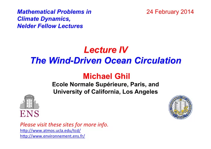
Mathematical Problems in 24 February 2014 Climate Dynamics, Nelder Fellow Lectures Lecture IV The Wind-Driven Ocean Circulation Michael Ghil Ecole Normale Suprieure, Paris, and University of California, Los Angeles Please visit
Mathematical Problems in 24 February 2014 Climate Dynamics, Nelder Fellow Lectures ¡ Lecture IV The Wind-Driven Ocean Circulation Michael Ghil Ecole Normale Supérieure, Paris, and University of California, Los Angeles � Please ¡visit ¡these ¡sites ¡for ¡more ¡info. ¡ h#p://www.atmos.ucla.edu/tcd/ ¡ h#p://www.environnement.ens.fr/ ¡ ¡
Motivation • The North Atlantic Oscillation (NAO) is a leading mode of variability of the Northern Hemisphere and beyond. � • It affects the atmosphere and oceans on several time and space scales. � • Its predictive understanding could help interannual and decadal-scale climate prediction over and around the North Atlantic basin. � • The hierarchical modeling approach allows one to � � give proper weight to the understanding provided by the � � models vs . their realism, respectively. � • Back-and-forth between “toy” (conceptual) and detailed (“realistic”) models , and between models and data . � Joint work with F. Codron, H. A. Dijkstra, Y. Feliks, S. Jiang, F.-F. Jin, � H. Le Treut, E. Simonnet, S. Speich , and S. Wang �
The NAO and the oceans ʼ wind-driven circulation � The low-frequency variability of the double-gyre circulation � �� – bifurcations in a toy model � � multiple equilibria, periodic and chaotic solutions � �� �� – some intermediate model results � Atmospheric impacts � �� – simple and intermediate models + GCMs � Some data analysis – atmospheric and oceanic � Some very promising NAO results � Conclusions and bibliography �
The NAO and the oceans ʼ wind-driven circulation � The low-frequency variability of the double-gyre circulation � �� – bifurcations in a toy model � � multiple equilibria, periodic and chaotic solutions � �� �� – some intermediate model results � Atmospheric impacts � �� – simple and intermediate models + GCMs � Some data analysis – atmospheric and oceanic � Some very promising NAO results � Conclusions and bibliography �
Positive phase Negative phase
An example of bifurcations and hierarchical An example of bifurcations and hierarchical modeling: The oceans’ ’ wind-driven circulation wind-driven circulation modeling: The oceans The mean surface currents are (largely) wind-driven
Monthly paths from altimeter: Stable vs. unstable periods
10-day sequences of subtropical jet paths: blocked vs. zonal flow regimes
The NAO and the oceans ʼ wind-driven circulation � The low-frequency variability of the double-gyre circulation � �� – bifurcations in a toy model � � multiple equilibria, periodic and chaotic solutions � �� �� – some intermediate model results � Atmospheric impacts � �� – simple and intermediate models + GCMs � Some data analysis – atmospheric and oceanic � Some very promising NAO results � Conclusions and bibliography �
Modeling Hierarchy for the Oceans Ocean models ♦ 0-D: box models – chemistry (BGC), paleo ♦ 1-D: vertical (mixed layer, thermocline) ♦ 2-D – meridional plane – THC → also 1.5-D: a little longitude dependence – horizontal – wind-driven → also 2.5-D: reduced-gravity models (n.5) ♦ 3-D: OGCMs - simplified - with bells & whistles (“kitchen sink”) Coupled 0-A models ♦ Idealized (0-D & 1-D): intermediate couple models (ICM) ♦ Hybrid (HCM) - diagnostic/statistical atmosphere - highly resolved ocean ♦ Coupled GCM (3-D): CGCM
The double-gyre circulation and its The double-gyre circulation and its low-frequency variability low-frequency variability An “intermediate” model of the mid-latitude, wind-driven ocean circulation: 20-km resolution, about 15 000 variables
The JJG model’ ’s s equilibria equilibria The JJG model Nonlinear (advection) effects break the (near) symmetry: (perturbed) pitchfork bifurcation? Subpolar gyre dominates Subtropical gyre dominates
Time-dependent solutions: Time-dependent solutions: periodic and chaotic periodic and chaotic To capture space- time dependence, meteorologists and oceanographers often use Hovmöller diagrams
Poor man’ ’s continuation method s continuation method Poor man
Interannual variability: variability: Interannual relaxation oscillation relaxation oscillation
Global bifurcations in Global bifurcations in “intermediate intermediate” ” models models “ Bifurcation tree in a QG, equivalent-barotropic, high-resolution (10 km) model: pitchfork, mode-merging, Hopf, and homoclinic
Homoclinic orbit: numerical and analytical orbit: numerical and analytical Homoclinic
The double-gyre circulation: The double-gyre circulation: A different rung of the hierarchy A different rung of the hierarchy Another “intermediate” model of the double-gyre circulation: slightly different physics, higher resolution – down to 10 km in the horizontal and more layers in the vertical, much larger domain, … Bo Qiu, U. of Hawaii, pers. commun., 1997
Model-to-model, qualitative comparison Model-to-model, qualitative comparison
Model-and-observations, Model-and-observations, quantitative comparison quantitative comparison Spectra of (a) kinetic energy of 2.5-layer shallow-water model in North-Atlantic– shaped basin; and (b) Cooperative Ocean- Atmosphere Data Set (COADS) Gulf-Stream axis data
Multi-channel SSA � analysis of the UK � Met Office monthly � mean SSTs for the � century-long � 1895–1994 interval � Marked similarity with the � 7–8-year “gyre mode” of � a full hierarchy of ocean � models, on the one hand, � and with the North � Atlantic Oscillation (NAO), � on the other: explanation? �
The NAO and the oceans ʼ wind-driven circulation � The low-frequency variability of the double-gyre circulation � �� – bifurcations in a toy model � � multiple equilibria, periodic and chaotic solutions � �� �� – some intermediate model results � Atmospheric impacts � �� – simple and intermediate models + GCMs � Some data analysis – atmospheric and oceanic � Some very promising NAO results � Conclusions and bibliography �
• H1 • H2 • AMBL A quasi-geostrophic (QG) atmospheric model in a periodic β -channel, first barotropic (Feliks et al ., JAS , 2004; FGS’04), then baroclinic (FGS’07). Marine atmospheric boundary layer (ABL), analytical solution. Forcing by idealized oceanic SST front.
Ocean-atmosphere coupling mechanism (II) Vertical velocity at the top of the marine ABL The nondimensional w ( H e ) is given by ❤ ✐ γζ g − α ∇ 2 T w ( H e ) = , with γ = c 1 ( f 0 L / U )( H e / H a ) and α = c 2 ( g / T 0 U 2 )( H 2 e / H a ) , where H a is the layer depth of the free atmosphere ( ∼ 10 km), and ζ g the atmospheric geostrophic vorticity. Two components: one mechanical , due to the geostrophic flow ζ g above the marine ABL and one thermal , induced by the SST front. Atmospheric jet t e j He c i n a e c SST O North South Michael Ghil, Eric Simonnet, Yizhak Feliks
30-day oscillation 70-day oscillation
Simulate atmospheric response to SODA data over the Gulf Stream region Use SST (–5 m) data from the SODA reanalysis (50 years) Use the FGS’07 QG model in periodic β -channel – baroclinic + marine ABL Figure shows NAO index: – simulated (solid) – observed (dashed)
Tipping points and bifurcations: do they really help? � � – Yes, if properly understood and carefully applied! � Can we predict them? � � – Yes, depending on the problem and the data! �
Slow amplitude modulation of 1 0 C in the SST front Low-energy phase High-energy phase
The NAO and the oceans ʼ wind-driven circulation � The low-frequency variability of the double-gyre circulation � �� – bifurcations in a toy model � � multiple equilibria, periodic and chaotic solutions � �� �� – some intermediate model results � Atmospheric impacts � �� – simple and intermediate models + GCMs � Some data analysis – atmospheric and oceanic � Some very promising NAO results � Conclusions and bibliography �
Waves vs. Particles: A Pathway to Prediction? Is predicting as hard � as it is claimed to be? � No, it’s actually quite easy: � Just flip a coin or roll a die! � What’s difficult, though, is � trusting the prediction � That’s where a little � understanding of what we’re � trying to predict helps! � Based on Ghil & Robertson (2002) �
Recommend
More recommend
Explore More Topics
Stay informed with curated content and fresh updates.
