Lecture 6. Poisson regression - Random points in space 1 Igor - PowerPoint PPT Presentation
Lecture 6. Poisson regression - Random points in space 1 Igor Rychlik Chalmers Department of Mathematical Sciences Probability, Statistics and Risk, MVE300 Chalmers April 2013 1 Section 7.1.2 is not included in the course. Counting number
Lecture 6. Poisson regression - Random points in space 1 Igor Rychlik Chalmers Department of Mathematical Sciences Probability, Statistics and Risk, MVE300 • Chalmers • April 2013 1 Section 7.1.2 is not included in the course.
Counting number of events N : Data: Suppose we have observed values of N 1 , . . . , N k , which are equal to n 1 , n 2 , . . . , n k , say. The first assumption is that N i are independent Poisson with constant mean m (the same as N has). Suppose that the test for over-disperion leads to rejection of the hypothesis that N i are iid Poisson. Overdispertion can be caused by variable mean of N i or that Poisson model is wrong. What can we do? The first step is to assume that N i are Poisson but have different expectations m i . Little help for predicting future unless one can model variability of m i !
Check Exposure: When we compared number of perished in traffic 1998 in US ( N US ) and Sweden ( N SE ) the numbers were very different (14500, 500, resp.). This was explained by different numbers of peoples leaving in the countries. In order to compare risks one tries to find a suitable measure of exposure to the hazard and study the rate of accidents 2 . For example in case of traffic a particularly useful measure of exposure is the total number of kilometers driven during a year. In other situations, e.g. in biology, one may count the number of tree species in a forest, and the rate would be the number of species per square kilometer. We found that 1998 the rate in US was about 1 person per 100 · 10 6 km driven while in Sweden, 1 per 125 · 10 6 km. The rates are close but (is the difference significant or could one assume that rates in both countries are the same?) 2 Rate is a count of events occurring to a particular unit of observation, divided by some measure of that unit’s exposure.
Simple case of two counts N 1 and N 2 : Suppose that N i ∈ Po ( m i ), i = 1 , 2. In general m 1 � = m 2 . There are two natural simple models for m i : ◮ Model I: m 1 = m 2 = m ◮ Model II: m 1 = λ t 1 and m 2 = λ t 2 . Here t 1 , t 2 are known exposures for the two counts. Two hypothesis are of interest: does the data contradicts Model I or Model II? If yes then and one draws conclusion that m 1 and m 2 need to be estimated separately. We will present a test quantity, called Deviance , which is a difference between values of the log-likelihoods for the compared models. Let first recall the ML-estimation of parameters in Poisson distribution.
Parametric modeling - log-likelihood l ( θ ) = ln( L ( θ )): Suppose N i ∈ Po ( m i ), i = 1 , . . . , k , are independent and that one has observed N i = n i . In general m i can take different values. Schema how to define log-likelihood function: → l ( m 1 , . . . , m k ) , 3 l ( θ ) : θ �− → ( m 1 , . . . , m k ) �− where θ is a parameter (or vector of parameters). Functions m i ( θ ) are models of the expected value variability. Examples: ◮ 1) θ = m , m i ( θ ) = m ; ◮ 2) θ = ( β 0 , β 1 ), m i ( θ ) = exp( β 0 + β 1 · i ) ◮ 3) θ = ( m 1 , . . . , m k ), m i ( θ ) = m i . 3 l ( m 1 , . . . , m k ) = � n i ln m i − � m i − � ln n i !
Finding ML-estimates θ ∗ of parameters: The ML-estimate θ ∗ of θ is the solution of equation system ˙ l ( θ ∗ ) = 0. For example: θ ∗ = � n i / k . ◮ 1) θ = m , ◮ 2) θ = ( β 0 , β 1 ), β ∗ 0 , β ∗ 1 has to be solved numerically. ◮ 3) θ = ( m 1 , . . . , m k ), i = n i . m ∗ Which model should one choose? Intuitively - likelihood corresponds to odds for parameters: if fraction of likelihood L ( θ 1 ) / L ( θ 2 ) >> 1 it means that we believe much more in the first values of parameters than in the second ones. Now L ( θ 1 ) / L ( θ 2 ) ≫ 1 ⇐ ⇒ ln( L ( θ 1 ) / L ( θ 2 )) = l ( θ 1 ) − l ( θ 2 ) ≫ 0
Deviance: Suppose we wish to choose between a simple model (marked s ) and more complex one (marked c ) (which include simpler model as a special case). θ c �− → ( m 1 ( θ c ) , . . . , m k ( θ c )) �− → l ( θ c ) , θ s �− → ( m 1 ( θ s ) , . . . , m k ( θ s )) �− → l ( θ s ) , The maximum likelihood of the parameters are θ ∗ s and θ ∗ c and the values of log likelihoods � � � l ( θ ∗ c ) = n i ln m i ( θ ∗ c ) − n i − ln n i ! . � � � l ( θ ∗ s ) = n i ln m i ( θ ∗ s ) − n i − ln n i ! s )) = 2 � n i (ln m i ( θ ∗ s )) > χ 2 If DEV = 2 ( l ( θ ∗ c ) − l ( θ ∗ c ) − ln m i ( θ ∗ α ( f ) then more complex model explains data better than the simpler one does (with approximative significance 1 − α ). Here f is the difference between the dimensions of θ c and θ s . In our example simple model has dimension 1 while the complex dimension k hence f = k − 1.
Numbers of perished in traffic 1998 in US and Sweden Let N US ∈ Po ( m US ), N SE ∈ Po ( m SE ). Observed numbers are about n US = 41500 while n SE = 500. Exposures were t US = 4 . 14 · 10 12 , t SE = 0 . 0625 · 10 12 [km], respectively. ◮ The ”simple model” postulates that the rates of fatal accidents are the same in both countries, i.e. m US = λ · t US and m SE = λ · t SE . λ ∗ = n US + n SE [km − 1 ] . = 0 . 9994 · 10 − 8 , t US + t SE ◮ The ”complex model” is that the rates are different, i.e. m US = λ US · t US and m SE = λ SE · t SE . US = n US SE = n SE = 1 . 000 · 10 − 8 , = 0 . 8 · 10 − 8 [km − 1 ] . λ ∗ λ ∗ t US t SE ( Deviance will be computed on the blackboard! ) 4 4 DEV = 27 . 51, f = 2 − 1, with α = 0 . 01, DEV > χ 2 α (1) = 6 . 635, we reject hypothesis that rates in US and Sweden are the same.
Numbers of railway accidents Authorities are interested in the impact of usage of different track types. Data consists of derailments of passenger trains 1 January 1985 – 1 May 1995. There were n 1 = 15 derailments on welded track with concrete sleepers and n 2 = 25 welded track with wooden sleepers . Assume that N 1 ∈ Po ( m con ) while N 2 ∈ Po ( m wod ) are independent. ◮ The ”simple model” is that m con = m wod = m m ∗ = n con + n wod = 20 . 2 ◮ The ”complex model” is that the means are different, i.e. m con � = m wod m ∗ con = n con = 15 , m ∗ wod = n wod = 25 . DEV = 2 · 15(ln 15 − ln 20) + 2 · 25(ln 25 − ln 20) = 2 . 53 < χ 2 0 . 05 (1) = 3 . 84 . The complex model is not better. Are both truck equally safe? 5 5 No , t con = 4 . 21 · 10 8 , t wod = 0 . 8 · 10 8 , [km], DEV = 40 . 9
Perished in traffic 1990-2000: N i - number of peoples killed in traffic year 1990 − 2000. t i - total driven distance, in 10 9 km, −8 1.25 x 10 800 1.2 750 1.15 1.1 700 1.05 650 1 0.95 600 0.9 0.85 550 0.8 500 1990 1992 1994 1996 1998 2000 1990 1992 1994 1996 1998 2000 Suppose that N i ∈ Po ( m ) (impossible but let test) ¯ n = 622 . 6 while s 2 k − 1 = 8487 . 5 then approximate confidence interval for V[ N ] / E[ N ] is χ 2 χ 2 1 − α/ 2 ( k − 1) α/ 2 ( k − 1) ¯ n ≤ V[ N ] n ¯ (0 . 024 =) E[ N ] ≤ (= 0 . 15) s 2 s 2 k − 1 k − 1 k − 1 k − 1
Modelling: Data: for i = − 5 , − 4 , . . . , 4 , 5: n i : [772 745 759 632 589 572 537 541 531 580] t i : [64 . 3 64 . 9 65 . 5 64 . 1 64 . 9 66 . 1 66 . 5 66 . 7 67 . 4 69 . 6 ] Modelling E[ N i ] = m i , viz. define a function: θ �− → ( m 1 , . . . , m k ): ◮ 1) θ s1 = ( β 0 , β 1 ), m i ( θ ) = exp( β 0 + β 1 · i ) ◮ 2) θ s2 = ( β 0 , β 1 , β 2 ), m i ( θ ) = exp( β 0 + β 1 · i + β 2 · t i ) ◮ 3) θ c = ( m 1 , . . . , m k ), m i ( θ ) = m i . ML-estimates are: ◮ ( β ∗ 0 , β ∗ 1 ) = (6 . 42 , − 0 . 0364) which means about 3% yearly decrease; ◮ ( β ∗ 0 , β ∗ 1 , β ∗ 2 ) = (0 . 85 , − 0 . 0828 , 0 . 084) which means about 8% yearly decrease but also 8% increase if the total driving length increases by 10 9 km during one year.
Choice of model: 800 DEV 1 = 2 ( l ( θ ∗ c ) − l ( θ ∗ s1 )) = 42 . 25 compare with χ 2 750 0 . 05 (9) = 16 . 92 (rejection of the simple model!). 700 650 DEV 2 = 2 ( l ( θ ∗ c ) − l ( θ ∗ s2 )) = 6 . 99 compare with χ 2 0 . 05 (8) = 15 . 51 (Good 600 model!). 550 500 1990 1992 1994 1996 1998 2000
A general Poisson process Let N ( B ) denote the number of events (or accidents) occurring in a region B . Consider the following list of assumptions: (A) More than one event can not happen simultaneously. (B) N ( B 1 ) is independent of N ( B 2 ) if B 1 and B 2 are disjoint. (C) Events happen in a stationary (time) and homogeneous (space) way, i.e. N ( B ) cdf depends only on size | B | of B . The process for which we can motivate that (A–B) are true is called a Poisson point process. It is a stationary (homogenous) process with constant intensity λ if (A–C) holds and N ( B ) ∈ Po( λ | B | ). × × × × × × × × B 2 × B 1 × × B Figure: N ( B ) = 11 while N ( B 1 ) = 2, N ( B 2 ) = 3.
Recommend
More recommend
Explore More Topics
Stay informed with curated content and fresh updates.
