
S02 - Poisson Regression STAT 401 (Engineering) - Iowa State - PowerPoint PPT Presentation
S02 - Poisson Regression STAT 401 (Engineering) - Iowa State University April 23, 2018 (STAT401@ISU) S02 - Poisson Regression April 23, 2018 1 / 20 Linear regression For continuous Y i , we have linear regression ind N ( i , 2 ) Y
S02 - Poisson Regression STAT 401 (Engineering) - Iowa State University April 23, 2018 (STAT401@ISU) S02 - Poisson Regression April 23, 2018 1 / 20
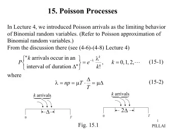
Linear regression For continuous Y i , we have linear regression ind ∼ N ( µ i , σ 2 ) Y i µ i = β 0 + β 1 X i, 1 + · · · + β p X i,p For binary or count with an upper maximum Y i , we have logistic regression ind Y i ∼ Bin ( n i , θ i ) � � θ i log = β 0 + β 1 X i, 1 + · · · + β p X i,p 1 − θ i What if Y i is a count without a maximum? (STAT401@ISU) S02 - Poisson Regression April 23, 2018 2 / 20
Poisson regression Poisson regression Let Y i ∈ { 0 , 1 , 2 , . . . } be a count (typically over some amount of time or some amount of space) with associated explanatory variables X i, 1 , . . . , X i,p . Then a Poisson regression model is ind Y i ∼ Po ( λ i ) and log( λ i ) = β 0 + β 1 X i, 1 + β 2 X i, 2 + · · · + β p X i,p (STAT401@ISU) S02 - Poisson Regression April 23, 2018 3 / 20
Poisson regression Interpretation When all explanatory variables are zero, then E [ Y i | X i, 1 = 0 , . . . , X i,p = 0] = λ i = e β 0 thus β 0 determines the expected response when all explanatory variables are zero. More generally, E [ Y i | X i, 1 = x 1 , . . . , X i,p = x p ] = e β 0 + β 1 x 1 + ··· + β p x p . If X i, 1 increases by one unit, we have E [ Y i | X i, 1 = x 1 +1 , . . . , X i,p = x p ] = e β 0 + β 1 ( x 1 +1)+ ··· + β p x p = e β 0 + β 1 x 1 + ··· + β p x p e β 1 Thus E [ Y i | X i, 1 = x 1 + 1 , . . . , X i,p = x p ] , . . . , X i,p = x p ] = e β 1 . E [ Y i | X i, 1 = x 1 Thus e β p is the multiplicative effect on the mean response for a one unit increase in the associated explanatory variable when holding all other explanatory variables constant. (STAT401@ISU) S02 - Poisson Regression April 23, 2018 4 / 20
Poisson regression Example Salamander habitat The Del Norte Salamander (plethodon elongates) is a small (57 cm) salamander found among rock rubble, rock outcrops and moss-covered talus in a narrow range of northwest California. To study the habitat characteristics of the species and particularly the tendency of these salamanders to reside in dwindling old-growth forests, researchers selected 47 sites from plausible salamander habitat in national forest and parkland. Randomly chosen grid points were searched for the presence of a site with suitable rocky habitat. At each suitable site, a 7 metre by 7 metre search are was examined for the number of salamanders it contained. (STAT401@ISU) S02 - Poisson Regression April 23, 2018 5 / 20
Poisson regression Example ggplot(Sleuth3::case2202, aes(ForestAge, Salamanders)) + geom_point() + theme_bw() 10 Salamanders 5 0 0 200 400 600 ForestAge (STAT401@ISU) S02 - Poisson Regression April 23, 2018 6 / 20
Poisson regression Example ggplot(Sleuth3::case2202, aes(ForestAge, log(Salamanders+1))) + geom_point() + theme_bw() 2 log(Salamanders + 1) 1 0 0 200 400 600 ForestAge (STAT401@ISU) S02 - Poisson Regression April 23, 2018 7 / 20
Poisson regression Example Analysis m <- glm(Salamanders ~ ForestAge, data = Sleuth3::case2202, family = "poisson") summary(m) Call: glm(formula = Salamanders ~ ForestAge, family = "poisson", data = Sleuth3::case2202) Deviance Residuals: Min 1Q Median 3Q Max -2.6970 -1.8539 -0.7987 0.2144 4.4582 Coefficients: Estimate Std. Error z value Pr(>|z|) (Intercept) 0.5040207 0.1401385 3.597 0.000322 *** ForestAge 0.0019151 0.0004155 4.609 4.05e-06 *** --- Signif. codes: 0 '***' 0.001 '**' 0.01 '*' 0.05 '.' 0.1 ' ' 1 (Dispersion parameter for poisson family taken to be 1) Null deviance: 190.22 on 46 degrees of freedom Residual deviance: 170.65 on 45 degrees of freedom AIC: 259.7 Number of Fisher Scoring iterations: 6 (STAT401@ISU) S02 - Poisson Regression April 23, 2018 8 / 20
Poisson regression Example ggplot(Sleuth3::case2202, aes(ForestAge, Salamanders)) + geom_point() + stat_smooth(method="glm", se=FALSE, method.args = list(family="poisson")) + theme_bw() 10 Salamanders 5 0 0 200 400 600 ForestAge (STAT401@ISU) S02 - Poisson Regression April 23, 2018 9 / 20
Poisson regression Multiple explanatory variables Salamander habitat (cont.) m <- glm(Salamanders ~ ForestAge * PctCover, data = Sleuth3::case2202, family = "poisson") summary(m) Call: glm(formula = Salamanders ~ ForestAge * PctCover, family = "poisson", data = Sleuth3::case2202) Deviance Residuals: Min 1Q Median 3Q Max -2.9710 -1.3237 -0.7378 0.6114 3.9136 Coefficients: Estimate Std. Error z value Pr(>|z|) (Intercept) -1.388e+00 5.038e-01 -2.754 0.00588 ** ForestAge -2.812e-03 6.799e-03 -0.414 0.67918 PctCover 3.147e-02 6.145e-03 5.121 3.04e-07 *** ForestAge:PctCover 3.141e-05 7.625e-05 0.412 0.68033 --- Signif. codes: 0 '***' 0.001 '**' 0.01 '*' 0.05 '.' 0.1 ' ' 1 (Dispersion parameter for poisson family taken to be 1) Null deviance: 190.22 on 46 degrees of freedom Residual deviance: 121.13 on 43 degrees of freedom AIC: 214.19 Number of Fisher Scoring iterations: 6 (STAT401@ISU) S02 - Poisson Regression April 23, 2018 10 / 20
Poisson regression Offset Offset If not all counts are based on the same amount of time or space, we need to account for the amount of time or space used. To do this, we can include an offset. Let T i represent the amount of time or space, then a Poisson regression model with an offset is ind Y i ∼ Po ( λ i ) and log( λ i ) = log( T i ) + β 0 + β 1 X i, 1 + β 2 X i, 2 + · · · + β p X i,p . The offset is log( T i ) and can be thought of as an explanatory variable with a known coefficient of 1. Note that log E [ Y i /T i ] = β 0 + β 1 X i, 1 + β 2 X i, 2 + · · · + β p X i,p so we are effectively modeling the rate. (STAT401@ISU) S02 - Poisson Regression April 23, 2018 11 / 20
Poisson regression Offset Airline crash data When considering airline crash data, we need to account for the fact that airlines are (typically) flying more miles year over year. airline = data.frame(year=1976:1985, fatal_accidents = c(24,25,31,31,22,21,26,20,16,22), passenger_deaths = c(734,516,754,877,814,362,764,809,223,1066), death_rate = c(0.19,0.12,0.15,0.16,0.14,0.06,0.13,0.13,0.03,0.15)) %>% mutate(miles_flown = passenger_deaths / death_rate) airline year fatal_accidents passenger_deaths death_rate miles_flown 1 1976 24 734 0.19 3863.158 2 1977 25 516 0.12 4300.000 3 1978 31 754 0.15 5026.667 4 1979 31 877 0.16 5481.250 5 1980 22 814 0.14 5814.286 6 1981 21 362 0.06 6033.333 7 1982 26 764 0.13 5876.923 8 1983 20 809 0.13 6223.077 9 1984 16 223 0.03 7433.333 10 1985 22 1066 0.15 7106.667 (STAT401@ISU) S02 - Poisson Regression April 23, 2018 12 / 20
Poisson regression Offset Visualize airline crash data ggplot(airline, aes(year, fatal_accidents)) + geom_point() + scale_x_continuous(breaks= scales::pretty_breaks()) + theme_bw() 28 fatal_accidents 24 20 16 1976 1978 1980 1982 1984 year (STAT401@ISU) S02 - Poisson Regression April 23, 2018 13 / 20
Poisson regression Offset Visualize airline crash data ggplot(airline, aes(year, fatal_accidents/miles_flown)) + geom_point() + scale_x_continuous(breaks= scales::pretty_breaks()) + theme_bw() 0.006 fatal_accidents/miles_flown 0.005 0.004 0.003 0.002 1976 1978 1980 1982 1984 year (STAT401@ISU) S02 - Poisson Regression April 23, 2018 14 / 20
Poisson regression Offset Offset in R m <- glm(fatal_accidents ~ year + offset(log(miles_flown)), data = airline, family = "poisson") summary(m) Call: glm(formula = fatal_accidents ~ year + offset(log(miles_flown)), family = "poisson", data = airline) Deviance Residuals: Min 1Q Median 3Q Max -1.2829 -0.5813 -0.1230 0.7254 1.0211 Coefficients: Estimate Std. Error z value Pr(>|z|) (Intercept) 201.32854 45.62354 4.413 1.02e-05 *** year -0.10442 0.02304 -4.532 5.84e-06 *** --- Signif. codes: 0 '***' 0.001 '**' 0.01 '*' 0.05 '.' 0.1 ' ' 1 (Dispersion parameter for poisson family taken to be 1) Null deviance: 26.133 on 9 degrees of freedom Residual deviance: 5.457 on 8 degrees of freedom AIC: 59.426 Number of Fisher Scoring iterations: 4 (STAT401@ISU) S02 - Poisson Regression April 23, 2018 15 / 20
Poisson regression Offset Offset in R m <- glm(fatal_accidents ~ year + log(miles_flown), data = airline, family = "poisson") confint(m) # No evidence coefficient for log(miles_flown) is incompatible with 1 2.5 % 97.5 % (Intercept) -134.5369352 415.57465599 year -0.2192575 0.07628503 log(miles_flown) -1.6508503 2.64154996 (STAT401@ISU) S02 - Poisson Regression April 23, 2018 16 / 20
Recommend
More recommend
Explore More Topics
Stay informed with curated content and fresh updates.













![Last time: iterated integrals (3 x 2 + 3 y 2 ) dA . Let D = [0 , 2] [ 3 , 1].](https://c.sambuz.com/795415/last-time-iterated-integrals-s.webp)
