Lecture 3: Convex Function CK Cheng Dept. of Computer Science and - PowerPoint PPT Presentation
CSE203B Convex Optimization: Lecture 3: Convex Function CK Cheng Dept. of Computer Science and Engineering University of California, San Diego 1 Outlines 1. Definitions: Convexity, Examples & Views 2. Conditions of Optimality 1. First
CSE203B Convex Optimization: Lecture 3: Convex Function CK Cheng Dept. of Computer Science and Engineering University of California, San Diego 1
Outlines 1. Definitions: Convexity, Examples & Views 2. Conditions of Optimality 1. First Order Condition 2. Second Order Condition 3. Operations that Preserve the Convexity 1. Pointwise Maximum 2. Partial Minimization 4. Conjugate Function 5. Log-Concave, Log-Convex Functions 2
Outlines 1. Definitions 1. Convex Function vs Convex Set 2. Examples 1. Norm 2. Entropy 3. Affine 4. Determinant 5. Maximum 3. Views of Functions and Related Hyperplanes 3
1. Definitions: Convex Function vs Convex Set Theorem: Given 𝑇 = 𝑦 𝑔 𝑦 ≤ 𝑐 If function 𝑔 𝑦 is convex, then 𝑇 is a convex set. Proof: We prove by the definition of convex set. For every 𝑣, 𝑤 ∈ 𝑇, i. e. 𝑔 𝑣 ≤ 𝑐, 𝑔 𝑤 ≤ 𝑐, We want to show that α𝑣 + 𝛾𝑤 ∈ 𝑇, ∀α + 𝛾 = 1, 𝛽, 𝛾 ≥ 0. We have 𝑔 𝛽𝑣 + 𝛾𝑤 ≤ 𝛽𝑔 𝑣 + 𝛾𝑔 𝑤 (𝑔 𝑗𝑡 𝑑𝑝𝑜𝑤𝑓𝑦) ≤ 𝛽𝑐 + 𝛾𝑐 (𝛽, 𝛾 ≥ 0) = 𝛽 + 𝛾 ∙ 𝑐 = 𝑐 (𝛽 + 𝛾 = 1) Thus α𝑣 + 𝛾𝑤 ∈ 𝑇 Remark: Convex function => Convex Set 𝑔(𝑦) ≤ 𝑐 => Convex Set 𝑔(𝑦) ≥ 𝑐 => ? 4
1. Convex Function Definitions: Examples 𝑔: 𝑆 𝑜 → 𝑆 is convex if 𝑒𝑝𝑛 𝑔 is a convex set and 𝑔 𝜄𝑦 + 1 − 𝜄 𝑧 ≤ 𝜄𝑔 𝑦 + 1 − 𝜄 𝑔(𝑧) ∀𝑦, 𝑧 ∈ 𝑒𝑝𝑛 𝑔, 0 ≤ 𝜄 ≤ 1 Example on R: Convex Functions 𝑏𝑦 + 𝑐 𝑝𝑜 𝑆 for any 𝑏, 𝑐 ∈ 𝑆 Affine: Exponential: 𝑓 𝑏𝑦 for any 𝑏 ∈ 𝑆 Power: 𝑦 𝛽 𝑝𝑜 𝑆 ++ for 𝛽 ≥ 1 or 𝛽 ≤ 0 𝑦 𝑞 𝑝𝑜 𝑆 for 𝑞 ≥ 1 Concave Functions 𝑏𝑦 + 𝑐 𝑝𝑜 𝑆 for any 𝑏, 𝑐 ∈ 𝑆 Affine: Power: 𝑦 𝛽 𝑝𝑜 𝑆 ++ for 0 ≤ 𝛽 ≤ 1 Logarithm: 𝑚𝑝𝑦 𝑝𝑜 𝑆 ++ 5
1. Convex Function Definitions: Examples Example on 𝑆 𝑜 : 𝑔 𝑦 = 𝑏 𝑈 𝑦 + 𝑐 Affine: 1 𝑞 𝑔𝑝𝑠 𝑞 ≥ 1; 𝑜 𝑦 𝑞 ൗ Norms: 𝑦 𝑞 = σ 𝑗=1 𝑦 ∞ = max |𝑦 𝑙 | 𝑙 Example on 𝑆 𝑛×𝑜 : 𝑛 σ 𝑘=1 𝑜 𝑔 𝑌 = 𝑢𝑠 𝐵 𝑈 𝑌 = σ 𝑗=1 𝐵 𝑗𝑘 𝑦 𝑗𝑘 Affine: Spectral (max singular value): 1 2 𝑌 2 = 𝜏 𝑛𝑏𝑦 𝑌 = (𝜇 𝑛𝑏𝑦 𝑌 𝑈 𝑌 ) Τ 𝑔 𝑌 = 6
1. Convex Function Definitions: Examples Concave Functions: 𝑜 Log Determinant: 𝑔 𝑌 = log det 𝑌 , 𝑒𝑝𝑛 𝑔 = S ++ 𝑊 ∈ 𝑇 𝑜 Proof: Let 𝑢 = 𝑔 𝑌 + 𝑢𝑊 𝑢 = 𝑚𝑝 𝑒𝑓𝑢 (𝑌 + 𝑢𝑊) = 𝑚𝑝 𝑒𝑓𝑢 𝑌 + 𝑚𝑝𝑒𝑓𝑢(𝐽 + 𝑢𝑌 − 1 2 𝑊𝑌 − 1 2 ) 𝑜 = 𝑚𝑝 𝑒𝑓𝑢 𝑌 + σ 𝑗=1 𝑚𝑝(1 + 𝑢𝜇 𝑗 ) 𝜇 𝑗 : 𝑓𝑗𝑓𝑜𝑤𝑏𝑚𝑣𝑓 𝑝𝑔 𝑌 − 1 2 𝑊𝑌 − 1 2 is concave in 𝑢 ⇒ 𝑔 is concave 7
Convex function examples: norm, max, expectation norm: If 𝑔: 𝑆 𝑜 → 𝑆 is a norm and 0 ≤ 𝜄 ≤ 1 𝑔 𝜄𝑦 + 1 − 𝜄 𝑧 ≤ 𝑔 𝜄𝑦 + 𝑔 1 − 𝜄 𝑧 triangle inequality = 𝜄𝑔(𝑦) + (1 − 𝜄)𝑔(𝑧) scalability 𝑦 𝑗 , 𝑦 = 𝑦 1 , 𝑦 2 , … , 𝑦 𝑜 𝑈 Max function: 𝑔 𝑦 = max 𝑗 𝑔 𝜄𝑦 + 1 − 𝜄 𝑧 = max 𝜄𝑦 𝑗 + 1 − 𝜄 𝑧 𝑗 𝑗 ≤ 𝜄 max 𝑦 𝑗 + 1 − 𝜄 max 𝑧 𝑗 𝑗 𝑗 = 𝜄𝑔 𝑦 + 1 − 𝜄 𝑔 𝑧 for 0 ≤ 𝜄 ≤ 1 Probability: (Expectation) If 𝑔 𝑦 is convex with 𝑞 𝑦 a probability at 𝑦, i. e. 𝑞 𝑦 ≥ 0, ∀𝑦 and 𝑞(𝑦) 𝑒𝑦 = 1 Then 𝑔 𝐹𝑦 ≤ 𝐹𝑔 𝑦 , where 𝐹𝑦 = 𝑦 𝑞 𝑦 𝑒𝑦 𝐹𝑔(𝑦) = 𝑔(𝑦) 𝑞 𝑦 𝑒𝑦 8
1.3 Views of Functions and Related Hyperplanes Given 𝑔 𝑦 , 𝑦 ∈ 𝑆 𝑜 , we plot the function in 𝑆 𝑜 and 𝑆 𝑜+1 spaces. 1. Draw function in 𝑆 𝑜 space 𝑦 𝑈 𝑦 − Equipotential surface: tangent plane 𝛼𝑔 𝑦 = 0 at 𝑦 2. Draw function in 𝑆 𝑜+1 space 2.1 Graph of function: {(𝑦, ℎ)|𝑦 ∈ 𝑒𝑝𝑛 𝑔, ℎ = 𝑔 𝑦 } 𝑦 𝑈 𝑦 − 𝐢𝐳𝐪𝐟𝐬𝐪𝐦𝐛𝐨𝐟 (h = 𝛼𝑔 𝑦 + 𝑔( 𝑦) ) 𝑦 𝑦 𝑦 𝑈 − 1 𝛼𝑔 ℎ − = 0 𝑔 𝑦 Example: 𝑔 𝑦 = 𝑦 2 . We show the hyperplane with 𝛼𝑔 𝑦 2.2. Epigraph: epi 𝑔 : {(x, 𝑢)|𝑦 ∈ 𝑒𝑝𝑛 𝑔, 𝑔 𝑦 ≤ 𝑢} A function is convex iff its epigraph is a convex set. Example: 𝑔 𝑦 = max 𝑔 𝑗 𝑦 | 𝑗 = 1 … 𝑠 , 𝑔 𝑗 𝑦 𝑏𝑠𝑓 𝑑𝑝𝑜𝑤𝑓𝑦. Since epi 𝑔 is the intersect of epi 𝑔 𝑗 , epi 𝑔 is convex. Thus, function 𝑔 is convex. 9
2. Conditions of Optimality: First Order Condition D efintion: 𝑔 is differentiable if 𝑒𝑝𝑛𝑔 is open and 𝜖𝑔 𝑦 𝜖𝑔 𝑦 𝜖𝑔 𝑦 𝛼𝑔(𝑦) ≡ ( 𝜖𝑦 1 , 𝜖𝑦 2 , … , 𝜖𝑦 𝑜 ) exists at each 𝑦 ∈ 𝑒𝑝𝑛𝑔 Theorem: Differentiable 𝑔 with convex domain is convex iff 𝑔 𝑧 ≥ 𝑔 𝑦 + 𝛼𝑔 𝑦 T 𝑧 − 𝑦 , ∀𝑦, 𝑧 ∈ 𝑒𝑝𝑛𝑔 Proof => If 𝑔 is convex 𝑈ℎ𝑓𝑜 1 − 𝑢 𝑔 𝑦 + 𝑢𝑔 𝑧 ≥ 𝑔 1 − 𝑢 𝑦 + 𝑢𝑧 , ∀0 ≤ 𝑢 ≤ 1 𝑢 𝑔 𝑧 − 𝑔 𝑦 ≥ 𝑔 𝑦 + 𝑢 𝑧 − 𝑦 − 𝑔(𝑦) 1 𝑔 𝑧 − 𝑔 𝑦 ≥ 𝑢 (𝑔 𝑦 + 𝑢 𝑧 − 𝑦 − 𝑔 𝑦 ) = 𝛼𝑔 𝑦 𝑧 − 𝑦 𝑥ℎ𝑓𝑜 𝑢 → 0 <= 𝐻𝑗𝑤𝑓𝑜 𝑔 𝑧 ≥ 𝑔 𝑦 + 𝛼𝑔 𝑦 T 𝑧 − 𝑦 , ∀𝑦, 𝑧 ∈ 𝑒𝑝𝑛𝑔 𝑀𝑓𝑢 𝑨 = 1 − 𝑢 𝑦 + 𝑢𝑧 where ൝ 𝑔 𝑦 ≥ 𝑔 𝑨 + 𝛼𝑔 𝑨 T 𝑦 − 𝑨 𝑔 𝑧 ≥ 𝑔 𝑨 + 𝛼𝑔 𝑨 T 𝑧 − 𝑨 Thus 1 − 𝑢 𝑔 𝑦 + 𝑢𝑔 𝑧 ≥ 𝑔(𝑨) 10
2. Conditions: Second Order Condition Definition: 𝑔 is twice differentiable if 𝑒𝑝𝑛𝑔 is open and the Hessian 𝛼 2 𝑔 𝑦 ∈ 𝑇 𝑜 𝜖 2 𝑔 𝑦 𝛼 2 𝑔 𝑦 𝑗𝑘 ≡ 𝜖𝑦 𝑗 𝜖𝑦 𝑘 , 𝑗, 𝑘 = 1, … , 𝑜 exists at each 𝑦 ∈ 𝑒𝑝𝑛𝑔 Theorem: Twice Differentiable 𝑔 with convex domain is convex iff 𝛼 2 𝑔 𝑦 ≽ 0, ∀𝑦 ∈ 𝑒𝑝𝑛𝑔 Proof: Using Lagrange remainder, we can find a z 𝑔 𝑦 + 𝑢(𝑧 − 𝑦) = 𝑔 𝑦 + 𝛼𝑔 𝑦 𝑈 𝑢 𝑧 − 𝑦 + 1 2 𝑢 2 𝑧 − 𝑦 𝑈 𝛼 2 𝑔 𝑨 𝑧 − 𝑦 , ∀0 ≤ 𝑢 ≤ 1, 𝑨 is between 𝑦 and 𝑦 + 𝑢(𝑧 − 𝑦) Since the last term is always positive by assumption, the first order condition is satisfied. 11
2. Conditions: Second Order Condition Example: Negative Entropy: 𝑔 𝑦 = 𝑦 log 𝑦 , 𝑦 ∈ 𝑆 ++ 𝑔 ′ 𝑦 = 𝑦 𝑦 + log 𝑦 = 1 + log 𝑦 , 𝑔 ′′ 𝑦 = 1 𝑦 Since 𝑦 ∈ 𝑆 ++ , 𝑔 ′′ 𝑦 > 0 ⇒ 𝑔 𝑦 is convex Show the plot of 𝑦 log 𝑦 Remark: • 1 st order condition can be used to design and prove the property of opt. algorithms. • 2 nd order condition implies the 1 st order condition • 2 nd order condition can be used to prove the convexity of the functions. 12
2. Conditions: Examples 1 2 𝑦 𝑈 𝑄𝑦 + 𝑟 𝑈 𝑦 + 𝑠, 𝑄 ∈ 𝑇 𝑜 • Quadratic Function: 𝑔 𝑦 = 𝛼𝑔 𝑦 = 𝑄𝑦 + 𝑟, 𝛼 2 𝑔 𝑦 = 𝑄 2 • Least Square: 𝑔 𝑦 = 𝐵𝑦 − 𝑐 2 𝛼𝑔 𝑦 = 2𝐵 𝑈 𝐵𝑦 − 𝑐 , 𝛼 2 𝑔 𝑦 = 𝐵 𝑈 𝐵 𝑦 2 • Quadratic over linear: 𝑔 𝑦, 𝑧 = 𝑧 , 𝑧 > 0 𝑈 𝑧 , − 𝑦 2 2𝑦 𝛼𝑔 𝑦, 𝑧 = , 𝑧 2 , 2 − 2𝑦 𝑧 2 = 2 𝑧 𝑧 𝛼 2 𝑔 𝑦 = 𝑧 −𝑦 2𝑦 2 −𝑦 𝑧 3 − 2𝑦 𝑧 2 𝑧 3 13
2. Conditions: Examples 𝑜 𝑓 𝑦 𝑙 (Smooth max of softmax • Log-sum-exp: 𝑔 𝑦 = log σ 𝐿=1 function) 1 1 𝛼 2 𝑔 𝑦 = 1 𝑈 𝑨 𝑨𝑨 𝑈 , 𝑨 𝑙 = 𝑓 𝑦 𝑙 1 𝑈 𝑨 𝑒𝑗𝑏 𝑨 − 1 𝑜 𝑜 2 𝑨 𝑗 − σ 𝑗=1 𝑜 𝑤 𝑈 𝛼 2 𝑔 𝑦 𝑤 = 𝑤 𝑗 𝑨 𝑗 2 ] ≥ 0, 1 𝑈 𝑨 2 [ σ 𝑗=1 σ 𝑗=1 𝑨 𝑗 𝑤 𝑗 for all 𝑤 ∈ 𝑆 𝑜 (Cauchy-Schwarz inequality) Thus, 𝑔(𝑦) is a convex function Cauchy-Schwarz inequality : 𝑏 𝑈 𝑏 𝑐 𝑈 𝑐 ≥ 𝑏 𝑈 𝑐 2 , 𝑏 𝑗 = 𝑨 𝑗 , 𝑐 𝑗 = 𝑤 𝑗 𝑨 𝑗 𝑏 𝑈 𝑐 𝑏 𝑈 𝑐 Proof 1: Let 𝑨 = 𝑏 − 𝑐 𝑈 𝑐 𝑐, or 𝑏 = 𝑨 + 𝑐 𝑈 𝑐 𝑐 We have a 𝑈 a = z T z + 𝑏 𝑈 𝑐 2 𝑐 𝑈 𝑐 2 𝑐 𝑈 𝑐 ≥ 𝑏 𝑈 𝑐 2 𝑐 𝑈 𝑐 2 𝑐 𝑈 𝑐 = 𝑏 𝑈 𝑐 2 𝑐 𝑈 𝑐 Proof 2: By induction 14
3. Operations that preserve convexity • Nonnegative multiple: 𝛽𝑔, where 𝛽 ≥ 0, 𝑔 is convex • Sum: 𝑔 1 + 𝑔 2 , where 𝑔 1 , 𝑏𝑜𝑒 𝑔 2 are convex • Composition with affine function: 𝑔 𝐵𝑦 + 𝑐 , where 𝑔 is convex 2 𝑔 𝐵𝑦 + 𝑐 = 𝐵 𝑈 𝛼 2 𝑔 𝑧|𝑧 = 𝐵𝑦 + 𝑐 𝐵 Proof: 𝛼 𝑦 𝑧 𝑛 log 𝑐 𝑗 − 𝑏 𝑗 𝑈 𝑦 𝑗 , E.g. 𝑔 𝑦 = − σ 𝑗=1 𝑈 𝑦 < 𝑐 𝑗 , 𝑗 = 1, … , 𝑛} 𝑒𝑝𝑛 𝑔 = {𝑦|𝑏 𝑗 𝑔 𝑦 = 𝐵𝑦 + 𝑐 (if 𝑔 is twice differentiable) 15
Recommend
More recommend
Explore More Topics
Stay informed with curated content and fresh updates.

