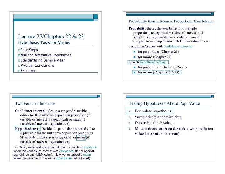

Probability then Inference, Proportions then Means Probability theory dictates behavior of sample proportions (categorical variable of interest) and Lecture 27/Chapters 22 & 23 sample means (quantitative variable) in random samples from a population with known values. Now Hypothesis Tests for Means perform inference with confidence intervals � Four Steps � for proportions (Chapter 20) � Null and Alternative Hypotheses � for means (Chapter 21) � Standardizing Sample Mean or with hypothesis testing � P -value, Conclusions � for proportions (Chapters 22&23) � Examples � for means (Chapters 22&23) Testing Hypotheses About Pop. Value Two Forms of Inference Confidence interval: Set up a range of plausible Formulate hypotheses. 1. values for the unknown population proportion (if Summarize/standardize data. 2. variable of interest is categorical) or mean (if Determine the P -value. variable of interest is quantitative). 3. Make a decision about the unknown population Hypothesis test: Decide if a particular proposed value 4. is plausible for the unknown population proportion value (proportion or mean). (if variable of interest is categorical) or mean (if variable of interest is quantitative). Last time, we tested about an unknown population proportion when the variable of interest was categorical (for or against gay civil unions, M&M color). Now we test about a mean when the variable of interest is quantitative (wt, IQ, cost).
Null and Alternative Hypotheses Standardizing Normal Values (Review) For a test about a single mean, Put a value of a normal distribution into perspective by standardizing to its z -score: � Null hypothesis: claim that the population mean equals a proposed value. observed value - mean � Alternative hypothesis: claim that the z = standard deviation population mean is greater, less, or not equal to a proposed value. The observed value that we need to standardize in this context is the sample mean . We’ve established Rules An alternative formulated with � is two-sided ; for its mean and standard deviation, and for when the with > or < is one-sided . shape is approximately normal, so that a probability (the P -value) can be assessed with the normal table. Conditions for Rule of Sample Means Rule for Sample Means (if conditions hold) � Randomness [affects center] � Center: The mean of sample means equals the � Independence [affects spread] true population mean. � If sampling without replacement, sample should be � Spread: The standard deviation of sample less than 1/10 population size means is standard error = Substitute sample � Large enough sample size [affects shape] standard deviation if population standard deviation � If population shape is normal, any sample size is OK population standard sample size � If population if not normal, a larger sample is needed. deviation is unknown. If 1st two conditions don’t hold, the mean and sd in z are � Shape: (Central Limit Theorem) The frequency wrong; if 3rd doesn’t hold, P -value is wrong. curve will be approximately normal, depending on how well 3rd condition is met.
Standardized Sample Mean P -value in Hypothesis Test about Mean � To test a hypothesis about an unknown population The P -value is the probability, assuming the null mean, find sample mean (and standard deviation) and hypothesis is true, of a sample mean at least as standardize to low/high/different as the one we observed. In sample mean - population mean particular, it depends on whether the alternative z = standard deviation hypothesis is formulated with a sample size less than, greater than, or not-equal sign. � z is called the test statistic . Note that “sample mean” is what we’ve observed, “population mean” is the value proposed in the null hypothesis, and “standard deviation” is from population (preferred) or sample (OK if sample size � 30). Making a Decision Based on a P -value Hypothesis Test for Means: Details If the P -value in our hypothesis test is small, our sample 1. null hypothesis: pop mean = proposed value mean is improbably low/high/different, assuming the alt hyp: pop mean < or > or � proposed value null hypothesis to be true. We conclude it is not true: 2. Find sample mean (and sd) and standardize to z . we reject the null hypothesis and believe the 3. Find the P -value= probability of sample mean as alternative. low/high/different as the one observed; same as If the P -value is not small, our sample mean is believable, probability of z this far below/above/away from 0. assuming the null hypothesis to be true. We are 4. If the P -value is small, conclude alternative is true. In willing to believe the null hypothesis. this case, we say the data are statistically significant P -value small reject null hypothesis (too extreme to attribute to chance). Otherwise, P -value not small don’t reject null hypothesis continue to believe the null hypothesis.
Example: Testing a Hypothesis about a Mean Example: Hypothesis Test about Smoking & IQ Background : Wts (in g) in a large colony of lab mice Background : IQs of children of a sample of 36 women � � have mean 30, sd 5. Grad students pick 25 “at random” who smoked while pregnant had mean 91. and find mean wt is 32.6. Question: Could this have been chance (null) or is it � Question: Was their sample actually biased? � significantly lower than pop mean IQ 100 (with sd 16)? Response: � Response: � Null: _________________ Alt: ___________________ 1. Null:__________________Alt:____________________ 1. Sample mean=____, sd=___, z = 2. Sample mean=___, pop sd=___, z = 2. P -value=prob of z this far below 0: ____________ 3. P -value=prob of z this far away from 0: ____________ 3. P -value is small, so reject null hypothesis. Conclude Because the P -value is __________________________ 4. 4. ___________________________________________ Conclude __________________________ Choosing the Right Display (Review) Choosing the Right Test Display type depends on variable types: Type of test depends on variable types: 1 measurement variable (students’ heights): stemplot, 1 categorical: z test about population proportion (done) � � boxplot, histogram, freq. curve (chs 7&8) 1 measurement (quan) [pop sd known or sample large]: � 1 categorical + 1 measurement var. (sex + ht): multiple z test about mean (done) � boxplots (ch 7, see p. 136) 1 measurement (quan) [pop sd unknown & sample small]: � 2 measurement variables: t test about mean (to do) � Time is expl (yr + cremation): time series (ch 15) 1 categorical (2 groups)+ 1 quan: two-sample z or t (to do) � � in general (age + wt): scatterplot (ch 10) � 2 categorical variables: chi-square test (done in Chapter 13) � 1 categorical var: (radio show type): piechart (ch 9) � 2 quan variables: regression test (not done in this course) � 2 or more cat vars (sex,smoke,on/off):barchart (ch 9) � (for 2 cat vars, use two-way table to organize data) Note: The t curve, like z , is bell-shaped and symmetric about 0. Because t has a bit more spread than z , our reaction to a t statistic is similar to what it would be for a z statistic but it takes a larger value of t to impress us, especially if the sample is small.
Example: t Test Two-Sample z or t Test Background : Cost (in $1000s) of coronary bypass surgery at a Null: mean for 1st population=mean for 2nd population � 1. sample of 9 hospitals had mean 24, sample sd 8. Two-sample t = 1st sample mean-2nd sample mean 2. Question: Are we convinced that the overall mean is >20? � 2 (1st sd) 2 (2nd sd) Response: + � 1st sample size 2nd sample size Null: ____________________ Alt: ______________________ 1. Obtain P -value based on z or t distribution Sample mean=___, sample sd=___, t = 3. 2. ( z for large samples, t for small samples). P -value = prob of t this far above 0 = ? 3. Note: the t curve is similar to z but more spread out: t values Reject null hypothesis if P -value is small. 4. must be more extreme to achieve significance. Since +1.5 is not large for z , ___________________________. 4. P -value is __________________________________________ ________________________ the population mean cost is more than 20 thousand dollars. Example: Two-Sample Test Chi-Square Test Background : Wait times (in seconds) at 7 banks on the west We learned to use chi-square to test for a relationship between two � coast had mean 231.6, sd 27.8, while 18 banks on the east coast categorical variables . had mean 272.7, sd 72.5. The two-sample t statistic was 2.05 Null hypothesis: the two variables are not related 1. and the P -value for a two-sided test was 0.052. Alternative hypothesis: the two variables are related 2 Question: Do mean wait times differ in general, east vs. west? � Test statistic=chi-square=(observed count-expected count) 2. Response: _______________________ Note that if z =2.05 � expected count (instead of t ), the P -value for a two-sided z test would be P -value= probability of chi-square this large, assuming the 3. ___________________, and the results would be somewhat two variables are not related. For a 2-by-2 table, more convincing. chi-square > 3.84 P -value < 0.05. If the P -value is small, conclude the variables are related. 4. Otherwise, we have no convincing evidence of a relationship. In general, a large test statistic is accompanied by a small P -value. Note: Next lecture we’ll do another example of a chi-square test.
Recommend
More recommend