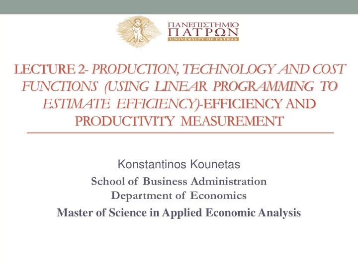
LECTURE 2- PRODUCTION, TECHNOLOGY AND COST FUNCTIONS (USING LINEAR - PowerPoint PPT Presentation
LECTURE 2- PRODUCTION, TECHNOLOGY AND COST FUNCTIONS (USING LINEAR PROGRAMMING TO ESTIMATE EFFICIENCY) -EFFICIENCY AND PRODUCTIVITY MEASUREMENT Konstantinos Kounetas School of Business Administration Department of Economics Master of
LECTURE 2- PRODUCTION, TECHNOLOGY AND COST FUNCTIONS (USING LINEAR PROGRAMMING TO ESTIMATE EFFICIENCY) -EFFICIENCY AND PRODUCTIVITY MEASUREMENT Konstantinos Kounetas School of Business Administration Department of Economics Master of Science in Applied Economic Analysis
Literature Review • Efficiency concepts developed by Farrell (1957); Fare, Grosskpof and Lovell (1985;1994); Lovell (1993). • Debreu (1951) and Koopmans (1951) defined simple measures of efficiency.
THE FUNDAMENTAL VIEW OF THE PROBLEM Inputs Outputs Transformation The units to be assessed transform inputs into outputs The basic requirement is to compare the Decision Making Units (DMUs) on the levels of outputs they secure relative to their input levels.
MEASURES OF COMPARATIVE EFFICIENCY Inputs Outputs Transformation In a given operating context the measure of efficiency is normally one of: - The distance between observed and maximum possible output for given inputs (output efficiency); - The distance between observed and minimum possible input for given outputs (input efficiency); - Remember that inputs and outputs are freely disposable
Efficiency Measures • Using the distance functions defined so far, we can define (Fare, Grosskopf and Lovell, 1994): • Technical efficiency • Allocative efficiency • Economic efficiency • A firm is said to be technically efficient if it operates on the frontier of the production technology • A firm is said to be allocatively efficient if it makes efficient allocation in terms of choosing optimal input and output combinations. • A firm is said to be economically efficient if it is both technically and allocatively efficient . • There is also the definition of scale efficiency (later on!!)
Input Orientated Measures I Lets assume a firm which is using two inputs (Labor and Capital) to produce s single output (Y- Total sales).The SS’ curve in the following Figure represents the knowledge of the unit isoquants of fully efficient firms. Technical Efficiency: TE I =OQ/OP=1-QP/OP X 2 /Y S Allocative Efficiency: AE I =OR/OQ P Economic Efficiency: EE I =OR/OP=1-QP/O EE I =AE I *TE I A Q All the measures are bounded between 0 and 1 Q’ R What TE=0.9 S’ means? O X 1 /Y
Input Orientated Measures II Farrell (1957) suggests the use of a non-parametric piece-wise-linear convex isoquant, 1. A parametric function (Cobb-Douglas) 2. By how much can input be proportionally X 2 /Y reduced without changing the output S produced? Can you form it in an another way? Piece-wise linear Unit Isoquant S’ O X 1 /Y
Output Orientated Measures I Y 1 /X 2 TE O =0A/0B AE O =0B/0C EE=0A/0C =TE O × AE O C • • B D • iso-revenue line • A PPC 0 Y 1 /X 1
A Simple Example Output B* Let us assume two firms A,B y* B with the following quantities y B B ( ) ( ) ( ) ( ) = = , 16,3 , , 64,7 x y x y A A B B A* y* A Can you calculate the average productivities and compare y A A the productivity index of firm A relative to firm B? How these measures are related with technical efficiency concept? O Input x A x B
Returns to Scale q q CRS Frontier VRS Frontier- DRTS D B D P A A B P C x C x
Returns to Scale • A production technology exhibits constant returns to scale (CRS) if a Z % increase in inputs results in Z % increase in outputs (ε = 1). • A production technology exhibits increasing returns to scale (IRS) if a Z % increase in inputs results in a more than Z % increase in outputs (ε > 1). • A production technology exhibits decreasing returns to scale (DRS) if a Z % increase in inputs results in a less than Z % increase in outputs (ε < 1).
Returns to scale q DRS CRS IRS x
Economies of scope • Is it less costly to produce M different products in one firm versus in M firms? • One measure of economies of scope is: M = − ( , ) ( , ) w w q c q c m = 1 m S ( , ) c w q • S > 0 implies economies of scope – it is better to produce the M outputs in one firm. • Other measures: • product specific measures • second derivative measures
Scale Efficiency • Productive efficiency is the combination of scale and technical. • Economic efficiency is the CRS Frontier combination of scale, technical and allocative. q VRS Frontier TE VRS =DB/DA TE CRS = DC/DA C • • • D A B SE=DC/DB = TE CRS /TE VRS x
Allocative Efficiency I labour • B isocost (420) A • isoquant (y=200) 0 capital isocost (360) AE=360/420=0.86
Allocative Efficiency II isocost (560) labour isocost (400) C • • A D isoquant (y=200) • • E TE=400/560=0.71 0 capital AE=360/400=0.9 isocost (360) CE=360/560=0.64
MOST PRODUCTIVE SCALE SIZE • Starrett (1977) generalize the concept of returns to scale in the context of multi-input, multi-output ( ) production function of two vectors , T x y dy n m T dx T + = j i 0 x y i j x x y y = = 1 1 i j i i j j • If we assume that all inputs-outputs increase at the same proportional rate α,β respectively we have a local measure of returns to scale = − = 1 DIR n T x dx i i x x = = − 1 i i i m dy T y j j y y = 1 j j j
MOST PRODUCTIVE SCALE SIZE • Banker defines most productive scale size with ( ) ( ) ( ) reference to if for any satisfying , T x y , x y , 1 • CRS holds at MPSS. • Banker also defines returns to scale measure as ( ) − 1 = lim − → 1 1
Methodology • There are two broad types of method for arriving at measures of comparative efficiency: parametric and non-parametric methods. • The parametric methods typically hypothesise a functional form and use the data to estimate the parameters of that function. The estimated function is then used to arrive at estimates of the efficiencies of units. • The non-parametric methods, best known as Data Envelopment Analysi s (DEA), create virtual units to act as benchmarks for measuring comparative efficiency.
The CRS DEA model y - column vector of outputs, q q MIN , x - column vector of inputs, − + . 0 s t y Y X - input matrix, i − θ 0 x X i Y - output matrix. q - efficiency score (q<=1). q < 1, inefficiency q = 1, efficiency Note: q is the measure of efficiency, given by the ratio between the weighted average of the outputs ( y ) produced and the weighted average of the inputs ( x ) used. See Coelli et al. (1998) for more details. The problem must been solved N times , one for each firm in the sample.
The VRS DEA model The CRS model can be easily modified to VRS by adding the n = convexity constraint that ensures that an inefficient firm is 1' 1 only “benchmarked” against firms of similar size. y - column vector of outputs, x - column vector of inputs, q MIN q , X - input matrix, − + s. to 0 y Y i Y - output matrix. q − 0 x X i q - efficiency score ( q< =1). = 1 ' 1 n 0 q < 1, inefficiency q = 1, efficiency Note: q is the measure of efficiency, given by the ratio between the weighted average of the outputs ( y ) produced and the weighted average of the inputs ( x ) used. See Coelli et al. (1998) for more details.
The VRS DEA model-Digging more I X 2 /Y • Slack • Define efficiency for S A,B firms. A • Is the point A’ a efficient point? A’ B • One could reduce the amount of X2 used by C the CA’ and produce B’ the same output (input D slack) S’ O X 1 /Y
The VRS DEA model-Digging more II x x y Firm x x 1 2 y y 1 2 1 1 2 5 2 5 2 2 2 4 1 2 3 3 6 6 2 2 4 1 3 2 3 2 5 2 6 2 3 1 • Input Slack equal to zero → − = 0 Y y i • Output Slack equal to zero → q − = 0 x X i http://www.uq.edu.au/economics/cepa/deap.php
The VRS DEA model-Digging more I Ι I x x y Firm x x 2 1 1 y 2 y 1 1 2 5 2 5 2 2 2 4 1 2 3 3 6 6 2 2 4 1 3 2 3 2 5 2 6 2 3 1 • Let us now for firm 3 see the LP problem!! min q q q , MIN ( ) − + + + + + . 0 , s t y y y y y y 3 1 1 2 2 3 3 4 4 5 5 − + ( ) q − + + + + . 0 s t y Y 0 x x x x x x 13 11 1 12 2 13 3 14 4 15 5 i ( ) q − + + + + − x x x x x x 0 θ 0 x X 23 21 1 22 2 23 3 24 4 25 5 i λ 0 ( ) ' = λ , , , , 1 2 3 4 5
The VRS DEA model-Digging more IV θ Firm IS OS IS 1 5 1 2 3 4 2 1 0.5 - 0.5 - - - - 0.5 - 2 1 - 1 - - - - - - 3 0.833 - 1 - - 0.5 - - - 4 0.714 - 0.214 - - 0.286 - - - 5 1 - - - - 1 - - - • Can you explain now the values of θ , λ? • What the value of technical efficiency say to us? • Which firms are the peers of firm 3? • Which firms are also the targets for firm 3?
Recommend
More recommend
Explore More Topics
Stay informed with curated content and fresh updates.
