Lecture 14: Shortest Paths Steven Skiena Department of Computer - PowerPoint PPT Presentation
Lecture 14: Shortest Paths Steven Skiena Department of Computer Science State University of New York Stony Brook, NY 117944400 http://www.cs.sunysb.edu/ skiena Problem of the Day Suppose we are given the minimum spanning tree T of a
Lecture 14: Shortest Paths Steven Skiena Department of Computer Science State University of New York Stony Brook, NY 11794–4400 http://www.cs.sunysb.edu/ ∼ skiena
Problem of the Day Suppose we are given the minimum spanning tree T of a given graph G (with n vertices and m edges) and a new edge e = ( u, v ) of weight w that we will add to G . Give an efficient algorithm to find the minimum spanning tree of the graph G + e . Your algorithm should run in O ( n ) time to receive full credit, although slower but correct algorithms will receive partial credit.
Shortest Paths Finding the shortest path between two nodes in a graph arises in many different applications: • Transportation problems – finding the cheapest way to travel between two locations. • Motion planning – what is the most natural way for a cartoon character to move about a simulated environment. • Communications problems – how look will it take for a message to get between two places? Which two locations are furthest apart, ie. what is the diameter of the network.
Shortest Paths and Sentence Disambiguation In our work on reconstructing text typed on an (overloaded) telephone keypad, we had to select which of many possible interpretations was most likely. We constructed a graph where the vertices were the possible words/positions in the sentence, with an edge between possible neighboring words.
� � ✣ ✢ ✛ ✚ ✙ ✜ ✗ ✗ ✗ ✖ ✪ ✖ ✖ ✕ ✕ ✕ ✔ ✔ ✔ ✏ ☛ ✦ ✙ ✑ ✙ ✗ ✗ ✗ ✗ ❏ ❏ ▲ ▲ ❏ ❏ ✫ ✫ ✙ ✪ ✦ ✣ ✢ ✛ ✚ ✙ ✜ ✙ ☛ ✗ ☛ ☛ ✖ ✕ ✕ ✕ ✔ ✔ ✔ ✏ ✑ ✖ ☛ ☞ ☛ � � � � � � ✖ ☛ ☛ � � � � ☞ � � � � ❂❄●✥◆P❖✰✁ ✬✭✬✮✬✰✯✲✱✳✱✵✴✷✶✷✸✳✹✷✶✷✸✳✺✷✸✷✻✼✱✵✹✽✱✾✯✿✬❀✬✭✬ ◗❙❘ ❚P❯✰❱❳❲✼❨❀❩❀❬P❭P❯✰❪ ❫❴❪ ❬P❯ ✁✄✂✆☎✞✝✠✟ ✁✄✂✆☎✄✝✠✟ ✁✄✂✆☎✞✝✠✟ ✁✄✂✆☎✞✝✡✟ ☞✍✌ ✎✍✏ ✎✍✏ ✒✍✏ ✓✍☞ ✑✍☞ ❵❛❚P❯✄❜✥❪ ❜✰❚❝❫❴❨❞❵❛❬P❯✄❡★❫★❢❴❣✄❩❀❫❴❪ ❬P❯ ✁✄✂✆☎✞✝✠✟ ✁✄✂✆☎✄✝✠✟ ✁✄✂✆☎✞✝✠✟ ✁✄✂✆☎✞✝✡✟ ☞✍✌ ✎✍✏ ✎✍✏ ✒✍✏ ✓✍☞ ✑✍☞ ✘✍✙ ✚✍✛ ✧★✙ ✩★✘ ✤✥✛ ✩★✘ ✩★✘ ❤❝❨✡❯✥❫❴❨✡❯✰❩❀❨❥✐✼❪ ❡❴❚❝❦♠❧✥❪ ❭P❣✄❚P❫❴❪ ❯✄❭ ✘✍✙ ✚✍✛ ▲❋▼ ✧★✙ ✩★✘ ❏❋❑ ❏❋❑ ✤✥✛ ✩★✘ ✩★✘ ♥✆❖✰✁✥◆❝❖✰✁ ❁✄❂❄❃✥❅❇❆✥❅❇❈❊❉❋❂✠●✄❁■❍
Weighting the Graph Code C 1 Code C 2 Code C 3 1 3 2 P(W /C ) P(W /C ) P(W /C ) 1 1 1 3 1 2 4 P(#/W ) 1 1 P(W /#) 1 2 1 1 P(W /W ) 3 P(W /C ) P(W /C ) 2 1 2 1 2 3 1 P(W /#) 2 2 # P(W /C ) # 2 2 1 P(W /#) 3 1 3 P(W /C ) P(W /C ) 1 3 3 3 1 P(W /#) 4 1 3 P(W /C ) P(W /C ) 3 4 1 4 The weight of each edge is a function of the probability that these two words will be next to each other in a sentence. ‘hive me’ would be less than ‘give me’, for example. The final system worked extremely well – identifying over 99% of characters correctly based on grammatical and statistical constraints.
Dynamic programming (the Viterbi algorithm) can be used on the sentences to obtain the same results, by finding the shortest paths in the underlying DAG.
Shortest Paths: Unweighted Graphs In an unweighted graph, the cost of a path is just the number of edges on the shortest path, which can be found in O ( n + m ) time via breadth-first search. In a weighted graph, the weight of a path between two vertices is the sum of the weights of the edges on a path. BFS will not work on weighted graphs because sometimes visiting more edges can lead to shorter distance, ie. 1 + 1 + 1 + 1 + 1 + 1 + 1 < 10 . Note that there can be an exponential number of shortest paths between two nodes – so we cannot report all shortest paths efficiently.
Negative Edge Weights Note that negative cost cycles render the problem of finding the shortest path meaningless, since you can always loop around the negative cost cycle more to reduce the cost of the path. Thus in our discussions, we will assume that all edge weights are positive. Other algorithms deal correctly with negative cost edges. Minimum spanning trees are uneffected by negative cost edges.
Dijkstra’s Algorithm The principle behind Dijkstra’s algorithm is that if s, . . . , x, . . . , t is the shortest path from s to t , then s, . . . , x had better be the shortest path from s to x . This suggests a dynamic programming-like strategy, where we store the distance from s to all nearby nodes, and use them to find the shortest path to more distant nodes.
Initialization and Update The shortest path from s to s , d ( s, s ) = 0 . If all edge weights are positive, the smallest edge incident to s , say ( s, x ) , defines d ( s, x ) . We can use an array to store the length of the shortest path to each node. Initialize each to ∞ to start. Soon as we establish the shortest path from s to a new node x , we go through each of its incident edges to see if there is a better way from s to other nodes thru x .
Pseudocode: Dijkstra’s Algorithm known = { s } for i = 1 to n , dist [ i ] = ∞ for each edge ( s, v ) , dist [ v ] = d ( s, v ) last= s while ( last � = t ) select v such that dist ( v ) = min unknown dist ( i ) for each ( v, x ) , dist [ x ] = min( dist [ x ] , dist [ v ] + w ( v, x )) last= v known = known ∪ { v } Complexity → O ( n 2 ) . This is essentially the same as Prim’s algorithm.
Dijkstra Example 5 7 2 6 2 4 5 9 3 3 5 7 1 7 4 2 4 12 A A G Dijkstra(G,A)
Dijkstra’s Implementation See how little changes from Prim’s algorithm! dijkstra(graph *g, int start) (* WAS prim(g,start) *) { int i; (* counter *) edgenode *p; (* temporary pointer *) bool intree[MAXV]; (* is the vertex in the tree yet? *) int distance[MAXV]; (* distance vertex is from start *) int v; (* current vertex to process *) int w; (* candidate next vertex *) int weight; (* edge weight *) int dist; (* best current distance from start *) for (i=1; i < = g − > nvertices; i++) { intree[i] = FALSE; distance[i] = MAXINT; parent[i] = -1; } distance[start] = 0; v = start;
while (intree[v] == FALSE) { intree[v] = TRUE; p = g − > edges[v]; while (p ! = NULL) { w = p − > y; weight = p − > weight; (* CHANGED *) if (distance[w] > (distance[v]+weight)) { (* CHANGED *) distance[w] = distance[v]+weight; (* CHANGED *) parent[w] = v; } p = p − > next; } v = 1; dist = MAXINT; for (i=1; i < = g − > nvertices; i++) if ((intree[i] == FALSE) && (dist > distance[i])) { dist = distance[i]; v = i; } } }
Prim’s/Dijkstra’s Analysis Finding the minimum weight fringe-edge takes O ( n ) time – just bump through fringe list. After adding a vertex to the tree, running through its adjacency list to update the cost of adding fringe vertices (there may be a cheaper way through the new vertex) can be done in O ( n ) time. Total time is O ( n 2 ) .
Improved Time Bounds An O ( m lg n ) implementation of Dijkstra’s algorithm would be faster for sparse graphs, and comes from using a heap of the vertices (ordered by distance), and updating the distance to each vertex (if necessary) in O (lg n ) time for each edge out from freshly known vertices. Even better, O ( n lg n + m ) follows from using Fibonacci heaps, since they permit one to do a decrease-key operation in O (1) amortized time.
All-Pairs Shortest Path Notice that finding the shortest path between a pair of vertices ( s, t ) in worst case requires first finding the shortest path from s to all other vertices in the graph. Many applications, such as finding the center or diameter of a graph, require finding the shortest path between all pairs of vertices. We can run Dijkstra’s algorithm n times (once from each possible start vertex) to solve all-pairs shortest path problem in O ( n 3 ) . Can we do better?
Dynamic Programming and Shortest Paths The four-step approach to dynamic programming is: 1. Characterize the structure of an optimal solution. 2. Recursively define the value of an optimal solution. 3. Compute this recurrence in a bottom-up fashion. 4. Extract the optimal solution from computed information.
Initialization From the adjacency matrix, we can construct the following matrix: D [ i, j ] = ∞ , if i � = j and ( v i , v j ) is not in E D [ i, j ] = w ( i, j ) , if ( v i , v j ) ∈ E D [ i, j ] = 0 , if i = j This tells us the shortest path going through no intermediate nodes.
Characterization Based on Path Length There are several ways to characterize the shortest path between two nodes in a graph. Note that the shortest path from i to j , i � = j , using at most M edges consists of the shortest path from i to k using at most M − 1 edges + W ( k, j ) for some k . This suggests that we can compute all-pair shortest path with an induction based on the number of edges in the optimal path.
Recommend
More recommend
Explore More Topics
Stay informed with curated content and fresh updates.
