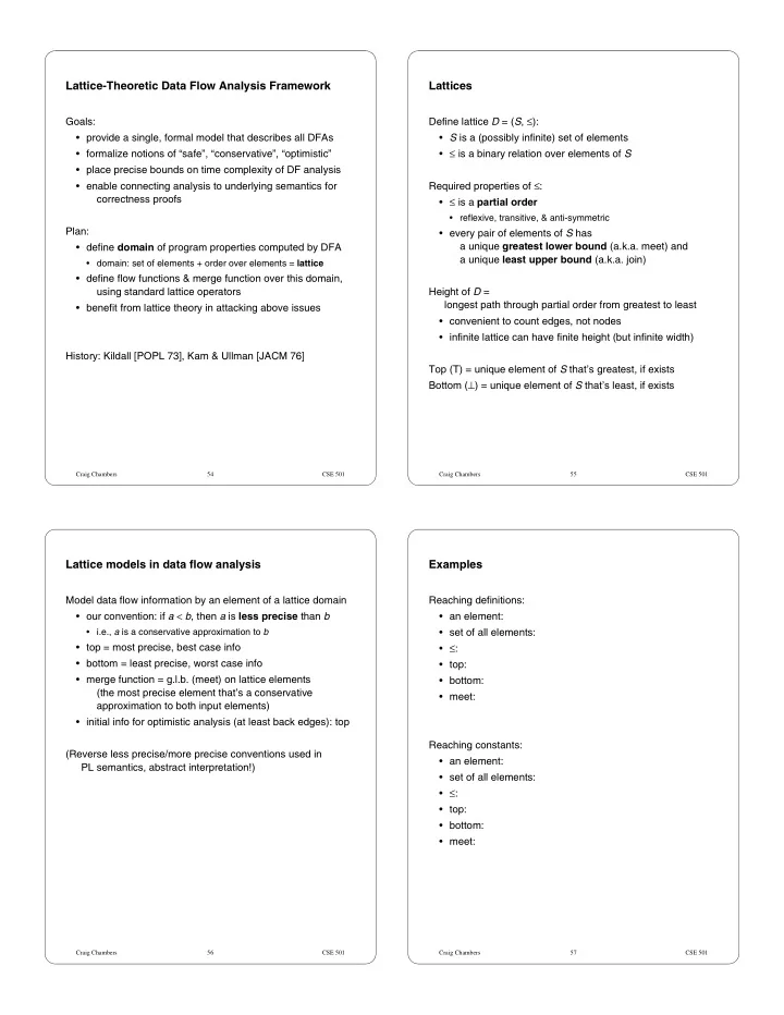
Lattice-Theoretic Data Flow Analysis Framework Lattices Define - PDF document

Lattice-Theoretic Data Flow Analysis Framework Lattices Define lattice D = ( S , ≤ ): Goals: • provide a single, formal model that describes all DFAs • S is a (possibly infinite) set of elements • ≤ is a binary relation over elements of S • formalize notions of “safe”, “conservative”, “optimistic” • place precise bounds on time complexity of DF analysis Required properties of ≤ : • enable connecting analysis to underlying semantics for correctness proofs • ≤ is a partial order • reflexive, transitive, & anti-symmetric Plan: • every pair of elements of S has a unique greatest lower bound (a.k.a. meet) and • define domain of program properties computed by DFA a unique least upper bound (a.k.a. join) • domain: set of elements + order over elements = lattice • define flow functions & merge function over this domain, using standard lattice operators Height of D = longest path through partial order from greatest to least • benefit from lattice theory in attacking above issues • convenient to count edges, not nodes • infinite lattice can have finite height (but infinite width) History: Kildall [POPL 73], Kam & Ullman [JACM 76] Top (T) = unique element of S that’s greatest, if exists Bottom ( ⊥ ) = unique element of S that’s least, if exists Craig Chambers 54 CSE 501 Craig Chambers 55 CSE 501 Lattice models in data flow analysis Examples Model data flow information by an element of a lattice domain Reaching definitions: • our convention: if a < b , then a is less precise than b • an element: • i.e., a is a conservative approximation to b • set of all elements: • ≤ : • top = most precise, best case info • bottom = least precise, worst case info • top: • merge function = g.l.b. (meet) on lattice elements • bottom: (the most precise element that’s a conservative • meet: approximation to both input elements) • initial info for optimistic analysis (at least back edges): top Reaching constants: (Reverse less precise/more precise conventions used in • an element: PL semantics, abstract interpretation!) • set of all elements: • ≤ : • top: • bottom: • meet: Craig Chambers 56 CSE 501 Craig Chambers 57 CSE 501

Some typical lattice domains Tuples of lattices Powerset lattice: set of all subsets of a set S Often helpful to break down a complex lattice into a tuple of • ordered by ⊆ or ⊇ lattices, one per variable/stmt/... being analyzed • top & bottom = ∅ & S , or vice versa Formally: D T = <S T , ≤ T > (D = <S, ≤ >) N = • height = | S | (infinite if S is infinite) • S T = S 1 × S 2 × ... × S N • “a collecting analysis” • element of tuple domain is a tuple of elements from each variable’s domain • i th component of tuple is info about i th variable/stmt/... A lifted set: a set of incomparable values, plus top & bottom • <..., d 1 i , ...> ≤ T <..., d 2 i , ...> ≡ d 1 i ≤ d 2 i , ∀ i • e.g., reaching constants domain, for a particular variable: • i.e. pointwise ordering T • meet: pointwise meet ... x=-2 x=-1 x=0 x=1 x=2 ... • top: tuple of tops ⊥ • bottom: tuple of bottoms • height(D T ) = N * height(D) • height = 2 [edges] (even though width is infinite!) Two-point lattice: top and bottom Powerset( S ) lattice is isomorphic to a tuple of two-point lattices, • computes a boolean property one two-point lattice element per element of S • i.e., a bit-vector! Single-point lattice: just bottom • trivial do-nothing analysis Craig Chambers 58 CSE 501 Craig Chambers 59 CSE 501 Example: reaching constants Analysis of loops in lattice model How to model reaching constants for all variables? Consider: d entry d backedge d head Informally: each element is a set of the form {..., x → k , ...}, with at most one binding for x B One lattice model: a powerset of all x → k bindings • S = pow({ x → k | ∀ x , ∀ k }) • ≤ = ⊆ (Assume B (d head ) computes d backedge ) • height? Want solution to constraints: Another lattice model: d head = d entry ∩ d backedge [ ∩ means meet] N -tuple of 3-level constant prop. lattices, for each of N variables d backedge = B (d head ) T Let F (d) = d entry ∩ B (d) ) N • ( ... x=-2 x=-1 x=0 x=1 x=2 ... ⊥ Then want fixed-point of F : • height? d head = F (d head ) If not, which is better? Craig Chambers 60 CSE 501 Craig Chambers 61 CSE 501

Iterative analysis in lattice model Termination of iterative analysis Iterative analysis computes fixed-point In general, k need not be finite by iterative approximation, beginning with T: Sufficient conditions for finiteness: F 0 = d entry ∩ T = d entry • flow functions (e.g. F ) are monotonic • lattice is of finite height F 1 = d entry ∩ B ( F 0 ) = F ( F 0 ) = F (d entry ) A function F is monotonic iff: F 2 = d entry ∩ B ( F 1 ) = F ( F 1 ) = F ( F ( F 0 )) = F ( F (d entry )) d 2 ≤ d 1 ⇒ F (d 2 ) ≤ F (d 1 ) • for application of DFA, this means that giving a flow function . . . at least as conservative inputs (d 2 ≤ d 1 ) leads to at least as conservative outputs ( F (d 2 ) ≤ F (d 1 )) F k = d entry ∩ B ( F k -1 ) = F ( F k -1 ) = F ( F (...( F (d entry ))...)) For monotonic F over domain D , the maximum number of times until that F can be applied to itself, starting w/ any element of D, w/o reaching fixed-point, is height( D ) F k +1 = d entry ∩ B ( F k ) = F ( F k ) F k = • start at top of D • for each application of F, either it’s a fixed-point, or the result must go down at least one level in lattice Is k finite? • eventually must hit a fixed-point If so, how big can it be? (which will be the best fixed-point) or bottom (which is guaranteed to be a fixed-point), if D of finite height Craig Chambers 62 CSE 501 Craig Chambers 63 CSE 501 Complexity of iterative analysis Another example: integer range analysis How long does iterative analysis take? For each program point, for each integer-typed variable, calculate (an approximation to) the set of integer values l : depth of loop nesting that can be taken on by the variable n : # of stmts in loop • use info for constant folding comparisons, t : time to execute one flow function for eliminating array bounds checks, k : height of lattice for (in)dependence testing of array accesses, for eliminating overflow checks What domain to use? • what is its height? What flow functions to use? • are they monotonic? Craig Chambers 64 CSE 501 Craig Chambers 65 CSE 501

Example Widening operators If domain is tall, then can introduce artificial generalizations for i := 0 to N-1 (called widenings ) when merging at loop heads ... a[i] ... end • ensure that only a finite number of widenings are possible • not easy to design the “right” widening strategy i := 0 i <= N-1? ... i >= 0 && i < N? t := a[i] ... i := i + 1 Craig Chambers 66 CSE 501 Craig Chambers 67 CSE 501 A generic worklist algorithm for lattice-theoretic DFA Maintain a mapping from each program point to info at that point • optimistically initialize all pp’s to T Set initial pp’s (e.g. entry/exit point) to their correct values Maintain a worklist of nodes whose flow functions need to be evaluated • initialize with all nodes in graph • include explicit meet (merge) & widening-meet (loop-head-merge) nodes While worklist nonempty do Remove a node from worklist Evaluate the node’s flow function, given current info on predecessor(successor) pp’s, allowing it to change info on successor(predecessor) pp’s If any pp info changed, put successor(predecessor) nodes on worklist (if not already there) For faster analysis, want to follow topological order • number nodes in forward(backward) topological order • remove nodes from worklist in increasing topological order Craig Chambers 68 CSE 501