Latent Semantic Indexing (LSI) CE-324: Modern Information Retrieval - PowerPoint PPT Presentation
Latent Semantic Indexing (LSI) CE-324: Modern Information Retrieval Sharif University of Technology M. Soleymani Spring 2020 Most slides have been adapted from: Profs. Manning, Nayak & Raghavan (CS-276, Stanford) Vector space model: pros
Latent Semantic Indexing (LSI) CE-324: Modern Information Retrieval Sharif University of Technology M. Soleymani Spring 2020 Most slides have been adapted from: Profs. Manning, Nayak & Raghavan (CS-276, Stanford)
Vector space model: pros } Partial matching of queries and docs } dealing with the case where no doc contains all search terms } Ranking according to similarity score } T erm weighting schemes } improves retrieval performance } Various extensions } Relevance feedback (modifying query vector) } Doc clustering and classification 2
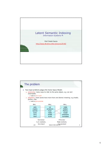
Problems with lexical semantics } Ambiguity and association in natural language } Polysemy : Words often have a multitude of meanings and different types of usage } More severe in very heterogeneous collections . } The vector space model is unable to discriminate between different meanings of the same word. 3
Problems with lexical semantics } Synonymy : Different terms may have identical or similar meanings (weaker: words indicating the same topic). } No associations between words are made in the vector space representation. 4
Polysemy and context } Doc similarity on single word level: polysemy and context ring jupiter ••• space voyager meaning 1 … … planet saturn ... ... car meaning 2 company ••• dodge contribution to similarity, if ford used in 1 st meaning, but not if in 2 nd 5
SVD Type equation here. 𝑊 2 𝑉 6
Latent Semantic Indexing (LSI) } Perform a low-rank approximation of doc-term matrix (typical rank 100-300) by SVD } latent semantic space } Term-doc matrices are very large but the number of topics that people talk about is small (in some sense) } General idea: Map docs (and terms) to a low-dimensional space } Design a mapping such that the low-dimensional space reflects semantic associations } Compute doc similarity based on the inner product in this latent semantic space 7
� Singular Value Decomposition (SVD) For an 𝑁 ´ 𝑂 matrix 𝐵 of rank 𝑠 there exists a factorization: 𝐵 = 𝑉Σ𝑊 2 𝑁 ´ 𝑁 𝑁 ´ 𝑂 𝑂 ´ 𝑂 𝑉 𝐵𝐵 𝑈 The columns of are orthogonal eigenvectors of . 𝑊 𝐵 𝑈 𝐵 The columns of are orthogonal eigenvectors of . l 1 l 𝑠 𝐵𝐵 𝑈 𝐵 𝑈 𝐵 Eigenvalues … of are also the eigenvalues of . Σ = diag 𝜏 > , … , 𝜏 A 𝜏 B = 𝜇 B Singular values Typically, the singular values arranged in decreasing order.
Singular Value Decomposition (SVD) 𝐵 = 𝑉Σ𝑊 2 } Truncated SVD min(𝑁, 𝑂) M ´ min( M,N) Min(M,N) ´ min(M, N) Min(M,N) ´ N min(𝑁, 𝑂) 9
� � � � � � � � � � � � � � � � � � � � � SVD example 1 −1 M= 3, N= 2 𝐵 = 0 1 1 0 0 2/ 6 1/ 3 1 0 1/ 2 1/√2 𝐵 = 1/ 2 −1/ 6 1/ 3 0 3 1/ 2 −1/ 2 0 0 1/ 2 −1/ 6 1/ 3 Or equivalently: 0 2/ 6 1 0 1/ 2 1/√2 1/ 2 −1/ 6 0 3 1/ 2 −1/ 2 1/ 2 −1/ 6
Example We use a non-weighted matrix here to simplify the example. 11
Example of 𝐷 = 𝑉Σ𝑊 2 : All four matrices 𝐷 = 𝑉Σ𝑊 𝑈 12
Example of 𝐷 = 𝑉Σ𝑊 2 : matrix 𝑉 One row per term One column per min( M , N ) Columns: “semantic” dims (distinct topics like politics, sports,...) 𝑣 𝑗𝑘 : how strongly related term 𝑗 is to the topic in column 𝑘 . 13
Example of 𝐷 = 𝑉Σ𝑊 2 : The matrix Σ square, diagonal matrix min( M , N ) × min( M , N ). Singular value: “measures the importance of the corresponding semantic dimension”. We’ll make use of this by omitting unimportant dimensions. 14
Example of 𝐷 = 𝑉Σ𝑊 2 : The matrix 𝑊 2 One column per doc One row per min( M , N ) Columns of 𝑊 : “semantic” dims 𝑤 𝑗𝑘 how strongly related doc 𝑗 is to the topic in column 𝑘 . : 15
Matrix decomposition: Summary } We’ve decomposed the term-doc matrix 𝐷 into a product of three matrices. } 𝑉 : consists of one (row) vector for each term } 𝑊 2 : consists of one (column) vector for each doc } Σ : diagonal matrix with singular values, reflecting importance of each dimension } Next:Why are we doing this? 16
Low-rank approximation } Solution via SVD 𝐵 V = 𝑉 diag 𝜏 > , … , 𝜏 V , 0, … 0 𝑊 2 set smallest r-k We retain only 𝑙 singular values singular values to zero 𝑙×𝑙 𝑙×𝑂 𝑁×𝑙 𝑁×𝑂 V column notation: 2 𝐵 V = W 𝜏 V 𝑣 B 𝑤 B sum of rank 1 matrices BX>
Low-rank approximation } SVD can be used to compute optimal low-rank approximations . } Keeping the 𝑙 largest singular values and setting all others to zero results in the optimal approximation [Eckart-Young]. } No matrix of the rank 𝑙 can approximates 𝐵 better than 𝐵 V . } Approximation problem : Given matrix 𝐵 , find matrix 𝐵 𝑙 of rank 𝑙 (e.g. a matrix with 𝑙 linearly independent rows or columns) such that 𝐵 V = [:A]^V [ XV 𝐵 − 𝑌 _ min Frobenius norm 𝐵 𝑙 and 𝑌 are both 𝑁×𝑂 matrices. Typically, we want 𝑙 ≪ 𝑠 . 18
Approximation error } How good (bad) is this approximation? } It’s the best possible, measured by the Frobenius norm of the error: [:A]^V [ XV 𝐵 − 𝑌 _ = min 𝐵 − 𝐵 V _ 𝐵 V = 𝑉 diag 𝜏 > , … , 𝜏 V , 0, … 0 𝑊 2 where the s 𝑗 are ordered such that s 𝑗 ³ s B`> . } Suggests why Frobenius error drops as 𝑙 increases. 19
SVD Low-rank approximation } Term-doc matrix 𝐷 may have 𝑁 = 50000 , 𝑂 = 10 b } rank close to 50000 } Construct an approximation 𝐷 100 with rank 100. } Of all rank 100 matrices, it would have the lowest Frobenius error. } Great … but why would we?? } Answer: Latent Semantic Indexing C. Eckart, G. Young, The approximation of a matrix by another of lower rank. Psychometrika, 1, 211-218, 1936.
Goals of LSI } SVD on the term-doc matrix } Similar terms map to similar location in low dimensional space } Noise reduction by dimension reduction 21
Term-document matrix This matrix is the basis for computing similarity between docs and queries. Can we transform this matrix, so that we get a better measure of similarity between docs and queries? . . . 22
Recall unreduced decomposition 𝐷 = 𝑉Σ𝑊 𝑈 23
Reducing the dimensionality to 2 24
Reducing the dimensionality to 2 25
Original matrix 𝐷 vs. reduced 𝐷 c = 𝑉Σ c 𝑊 2 𝐷 2 as a two - dimensional representation of 𝐷 . Dimensionality reduction to two dimensions. 26
Why is the reduced matrix “better”? Similarity of d2 and d3 in the original space: 0. Similarity of d2 und d3 in the reduced space: 0.52 * 0.28 + 0.36 * 0.16 + 0.72 * 0.36 + 0.12 * 0.20 + - 0.39 * - 0.08 ≈ 0.52 27 27
Why the reduced matrix is “better”? “boat” and “ship” are semantically similar. The “reduced” similarity measure reflects this. What property of the SVD reduction is responsible for improved similarity? 28
Example 29 [Example from Dumais et. al]
Example 30 [Example from Dumais et. al]
Example (k=2) 2 Σ V 𝑊 V 𝑉 V 31 [Example from Dumais et. al]
graph Squares: terms tree Circles: docs minor survey time response user computer interface human EPS system 32
33 [Example from Dumais et. al]
LSI: Summary } Decompose term-doc matrix 𝐷 into a product of matrices using SVD 𝐷 = 𝑉Σ𝑊 2 } We use columns of matrices 𝑉 and 𝑊 that correspond to the largest values in the diagonal matrix Σ as term and document dimensions in the new space 34
How we use the SVD in LSI } Key property of SVD: Each singular value tells us how important its dimension is. } By setting less important dimensions to zero, we keep the important information, but get rid of the “details”. } These details may } be noise ⇒ reduced LSI is a better representation } Details make things dissimilar that should be similar ⇒ reduced LSI is a better representation because it represents similarity better. 35
How LSI addresses synonymy and semantic relatedness? } Docs may be semantically similar but are not similar in the vector space (when we talk about the same topics but use different words). } Desired effect of LSI: Synonyms contribute strongly to doc similarity. } Standard vector space: Synonyms contribute nothing to doc similarity. } LSI (via SVD) selects the “least costly” mapping: } different words (= different dimensions of the full space) are mapped to the same dimension in the reduced space. } Thus, it maps synonyms or semantically related words to the same dimension. } “cost” of mapping synonyms to the same dimension is much less than cost of collapsing unrelated words. } Thus, LSI will avoid doing that for unrelated words. 36
Performing the maps } Each row and column of 𝐷 gets mapped into the 𝑙 - dimensional LSI space, by the SVD. } A query 𝑟 is also mapped into this space, by 𝑟 𝑙 = Σ V 2 𝑟 i> 𝑉 V h = Σ V i> 𝑉 V 2 𝐷 V , we Since V g should transform query 𝑟 to 𝑟 𝑙 } Query NOT a sparse vector. } Claim: this is not only the mapping with the best (Frobenius error) approximation to 𝐷 , but also improves retrieval. 37
Recommend
More recommend
Explore More Topics
Stay informed with curated content and fresh updates.
