Large shocks in menu cost models Peter Karadi Adam Reiff European - - PowerPoint PPT Presentation

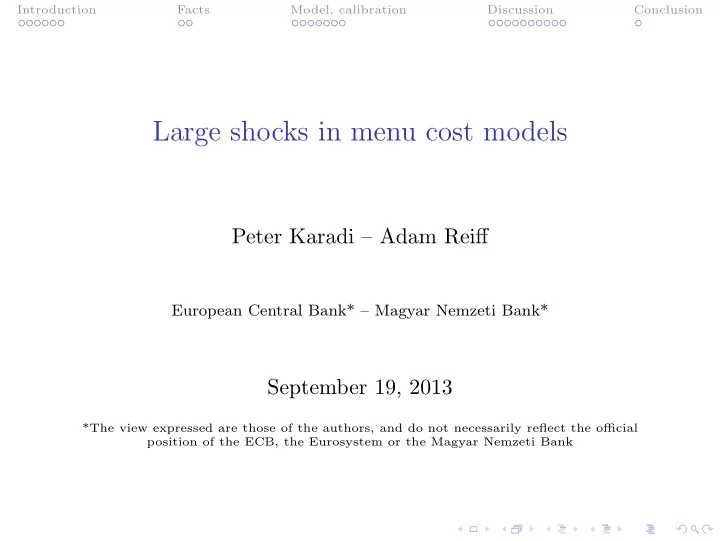
Introduction Facts Model, calibration Discussion Conclusion

Large shocks in menu cost models

Peter Karadi – Adam Reiff

European Central Bank* – Magyar Nemzeti Bank*

September 19, 2013

*The view expressed are those of the authors, and do not necessarily reflect the official position of the ECB, the Eurosystem or the Magyar Nemzeti Bank

Introduction Facts Model, calibration Discussion Conclusion

New-Keynesian Models

◮ Assume Calvo price stickiness

◮ timing of firms’ price adjustments is random

Introduction Facts Model, calibration Discussion Conclusion

New-Keynesian Models

◮ Assume Calvo price stickiness

◮ timing of firms’ price adjustments is random

◮ Claim: similar implications as in more micro-founded menu

cost models

◮ similarity in terms of aggregate price rigidity ◮ firms choose timing of price adjustments

Introduction Facts Model, calibration Discussion Conclusion

Debate

◮ Is Calvo indeed good approximation of menu cost models?

Introduction Facts Model, calibration Discussion Conclusion

Debate

◮ Is Calvo indeed good approximation of menu cost models? ◮ Golosov-Lucas (2007): No

◮ calibrate to micro price data ◮ match frequency, average size of price changes (∆p) ◮ aggregate price is flexible ◮ because of selection of price changers ◮ money essentially neutral

Introduction Facts Model, calibration Discussion Conclusion

Debate

◮ Is Calvo indeed good approximation of menu cost models? ◮ Golosov-Lucas (2007): No

◮ calibrate to micro price data ◮ match frequency, average size of price changes (∆p) ◮ aggregate price is flexible ◮ because of selection of price changers ◮ money essentially neutral

◮ Midrigan (2011): Yes

◮ match leptokurtic shape of ∆p-distribution ◮ by adding fat-tailed (rather than normal) shocks ◮ aggregate price rigidity similar to Calvo ◮ selection disappears

Introduction Facts Model, calibration Discussion Conclusion

Large shocks

◮ These results are for small shocks

◮ calibrated to nominal shocks during normal times

Introduction Facts Model, calibration Discussion Conclusion

Large shocks

◮ These results are for small shocks

◮ calibrated to nominal shocks during normal times

◮ What happens if shocks get large?

◮ large monetary shocks ◮ large devaluations ◮ large credit contractions ◮ tax changes

Introduction Facts Model, calibration Discussion Conclusion

Our paper

◮ Introduce new generalized menu cost model

◮ match distribution of ∆p even better

Introduction Facts Model, calibration Discussion Conclusion

Our paper

◮ Introduce new generalized menu cost model

◮ match distribution of ∆p even better

◮ Analyze model response to large monetary shocks

◮ compare with Calvo, Golosov-Lucas and Midrigan

Introduction Facts Model, calibration Discussion Conclusion

Our paper

◮ Introduce new generalized menu cost model

◮ match distribution of ∆p even better

◮ Analyze model response to large monetary shocks

◮ compare with Calvo, Golosov-Lucas and Midrigan

◮ Use micro data from Hungary to evaluate models

◮ Hungary: large, positive and negative (symmetric) tax

shocks

Introduction Facts Model, calibration Discussion Conclusion

Findings

◮ Aggregate price flexibility

Figure ◮ fraction of adjusters quickly increases with shock size ◮ =

⇒ inflation PT also increases quickly

◮ model with fat tailed shocks more flexible ◮ opposite of Midrigan’s small shock result

Introduction Facts Model, calibration Discussion Conclusion

Findings

◮ Aggregate price flexibility

Figure ◮ fraction of adjusters quickly increases with shock size ◮ =

⇒ inflation PT also increases quickly

◮ model with fat tailed shocks more flexible ◮ opposite of Midrigan’s small shock result

◮ Asymmetry

Figure ◮ asymmetric inflation PT for positive and negative shocks ◮ if there is trend inflation (small, 2% per year enough) ◮ negative shock: inflation takes care of price decreases ◮ model with fat tailed shocks more asymmetric

Introduction Facts Model, calibration Discussion Conclusion

Findings (cntd)

◮ Quantitative predictions of different models (in terms of

aggregate price flexibility and asymmetry)

◮ baseline model quite close to data ◮ normal model (GL) underestimates both ◮ leptokurtic model (M) overestimates both

Introduction Facts Model, calibration Discussion Conclusion

Findings (cntd)

◮ Quantitative predictions of different models (in terms of

aggregate price flexibility and asymmetry)

◮ baseline model quite close to data ◮ normal model (GL) underestimates both ◮ leptokurtic model (M) overestimates both

◮ Implication for small shocks

◮ baseline model is NOT similar to Calvo! ◮ Golosov-Lucas-type selection is back

Introduction Facts Model, calibration Discussion Conclusion

VAT-changes in Hungary

◮ 2006 January: decrease standard 25% VAT-rate to 20%

◮ pre-announced by 5 months

Introduction Facts Model, calibration Discussion Conclusion

VAT-changes in Hungary

◮ 2006 January: decrease standard 25% VAT-rate to 20%

◮ pre-announced by 5 months

◮ 2006 September: increase lower 15% VAT-rate to 20%

◮ pre-announced by 3 months

Introduction Facts Model, calibration Discussion Conclusion

VAT-changes in Hungary

◮ 2006 January: decrease standard 25% VAT-rate to 20%

◮ pre-announced by 5 months

◮ 2006 September: increase lower 15% VAT-rate to 20%

◮ pre-announced by 3 months

◮ Large and symmetric aggregate shocks

◮ affected different products ◮ use processed food sector ◮ increase- and decrease-affected products similar Moments

Introduction Facts Model, calibration Discussion Conclusion

Effects of VAT-changes

◮ Frequency of price change

◮ normal times (no tax change): 13.5% ◮ tax increase: 62% ◮ tax decrease: 26.9%

Introduction Facts Model, calibration Discussion Conclusion

Effects of VAT-changes

◮ Frequency of price change

◮ normal times (no tax change): 13.5% ◮ tax increase: 62% ◮ tax decrease: 26.9%

◮ Inflation pass-through (πt − ¯

π)/∆τt

◮ tax increase: 98.9% ◮ tax decrease: 32.9% ◮ aggregate price flexibility and asymmetry

Introduction Facts Model, calibration Discussion Conclusion

Effects of VAT-changes

◮ Frequency of price change

◮ normal times (no tax change): 13.5% ◮ tax increase: 62% ◮ tax decrease: 26.9%

◮ Inflation pass-through (πt − ¯

π)/∆τt

◮ tax increase: 98.9% ◮ tax decrease: 32.9% ◮ aggregate price flexibility and asymmetry

◮ Which sticky price model can predict this?

◮ Calvo surely not ◮ neither flexible nor asymmetric ◮ any of the menu cost models?

Introduction Facts Model, calibration Discussion Conclusion

Framework

◮ General equilibrium macro model with

◮ representative household ◮ heterogenous firms ◮ central bank and government (money growth and tax rates)

Introduction Facts Model, calibration Discussion Conclusion

Framework

◮ General equilibrium macro model with

◮ representative household ◮ heterogenous firms ◮ central bank and government (money growth and tax rates)

◮ Representative household

Equations ◮ maximizes lifetime utility in consumption aggregate (CES),

labor supply and real money balances

◮ standard CES-demand: Ct(i)/Ct = (Pt(i)/Pt)−θ

Introduction Facts Model, calibration Discussion Conclusion

Framework

◮ General equilibrium macro model with

◮ representative household ◮ heterogenous firms ◮ central bank and government (money growth and tax rates)

◮ Representative household

Equations ◮ maximizes lifetime utility in consumption aggregate (CES),

labor supply and real money balances

◮ standard CES-demand: Ct(i)/Ct = (Pt(i)/Pt)−θ

◮ Heterogenous firms

◮ hit by idiosyncr. productivity shocks (a la Golosov-Lucas) ◮ fat-tailed shocks to match empirical distribution of ∆p ◮ (more details on firms later)

Introduction Facts Model, calibration Discussion Conclusion

Framework

◮ General equilibrium macro model with

◮ representative household ◮ heterogenous firms ◮ central bank and government (money growth and tax rates)

◮ Representative household

Equations ◮ maximizes lifetime utility in consumption aggregate (CES),

labor supply and real money balances

◮ standard CES-demand: Ct(i)/Ct = (Pt(i)/Pt)−θ

◮ Heterogenous firms

◮ hit by idiosyncr. productivity shocks (a la Golosov-Lucas) ◮ fat-tailed shocks to match empirical distribution of ∆p ◮ (more details on firms later)

◮ Central bank and government

◮ passive: keep money growth (gM) and VAT-rate (τt) fixed ◮ unexpected change in money growth rate / VAT ◮ possibly pre-announced

Introduction Facts Model, calibration Discussion Conclusion

Heterogenous firms

◮ Continuum of firms (0 ≤ i ≤ 1), producing differentiated

products

◮ engage in monopolistic competition ◮ post prices Pt(i) ◮ pay fixed adjustment cost for each change in nominal price

Introduction Facts Model, calibration Discussion Conclusion

Heterogenous firms

◮ Continuum of firms (0 ≤ i ≤ 1), producing differentiated

products

◮ engage in monopolistic competition ◮ post prices Pt(i) ◮ pay fixed adjustment cost for each change in nominal price

◮ Single-input CRS technologies: Yt(i) = At(i)Lt(i)

◮ At(i) idiosyncratic productivity ◮ Lt(i) labor input

Introduction Facts Model, calibration Discussion Conclusion

Heterogenous firms

◮ Continuum of firms (0 ≤ i ≤ 1), producing differentiated

products

◮ engage in monopolistic competition ◮ post prices Pt(i) ◮ pay fixed adjustment cost for each change in nominal price

◮ Single-input CRS technologies: Yt(i) = At(i)Lt(i)

◮ At(i) idiosyncratic productivity ◮ Lt(i) labor input

◮ Log-productivity follows RW: ∆ log At(i) = εt(i)

Introduction Facts Model, calibration Discussion Conclusion

Heterogenous firms

◮ Continuum of firms (0 ≤ i ≤ 1), producing differentiated

products

◮ engage in monopolistic competition ◮ post prices Pt(i) ◮ pay fixed adjustment cost for each change in nominal price

◮ Single-input CRS technologies: Yt(i) = At(i)Lt(i)

◮ At(i) idiosyncratic productivity ◮ Lt(i) labor input

◮ Log-productivity follows RW: ∆ log At(i) = εt(i) ◮ Why have idiosyncratic productivity shocks?

◮ to match large size of price changes in data ◮ aggregate shocks with small inflation rate could not do this

Introduction Facts Model, calibration Discussion Conclusion

Heterogenous firms (cntd)

◮ Productivity innovation εt(i) is mixed normal

εt(i) = N(0, σ2/λ) with probability p N(0, σ2) with probability 1 − p

Introduction Facts Model, calibration Discussion Conclusion

Heterogenous firms (cntd)

◮ Productivity innovation εt(i) is mixed normal

εt(i) = N(0, σ2/λ) with probability p N(0, σ2) with probability 1 − p

◮ Special cases nested

◮ normal innovations a la Golsov-Lucas (2007) (p = 0) ◮ poisson innovations a la Midrigan (2011) (λ = ∞)

Introduction Facts Model, calibration Discussion Conclusion

Heterogenous firms (cntd)

◮ Productivity innovation εt(i) is mixed normal

εt(i) = N(0, σ2/λ) with probability p N(0, σ2) with probability 1 − p

◮ Special cases nested

◮ normal innovations a la Golsov-Lucas (2007) (p = 0) ◮ poisson innovations a la Midrigan (2011) (λ = ∞)

◮ Firms solve a dynamic problem of whether or not to

change price

Equations ◮ problem stationary in productivity adjusted relative price:

pt(i) = Pt(i)At(i)

Pt

Introduction Facts Model, calibration Discussion Conclusion

Equilibrium and numerical solution

◮ Standard equilibrium

Details ◮ agent maximize, given their information ◮ markets clear

Introduction Facts Model, calibration Discussion Conclusion

Equilibrium and numerical solution

◮ Standard equilibrium

Details ◮ agent maximize, given their information ◮ markets clear

◮ Numerical solution

◮ no aggregate uncertainty (tax, money growth rates fixed) ◮ steady state: global heterogenous agents methods Details ◮ transition dynamics: shooting Details

Introduction Facts Model, calibration Discussion Conclusion

Data

◮ Store-level monthly price data on processed food products

◮ 128 different products ◮ 123 stores/product on average ◮ time span: 2001 December – 2006 December ◮ product-level statistics, aggregated by CPI-weights

Introduction Facts Model, calibration Discussion Conclusion

Data

◮ Store-level monthly price data on processed food products

◮ 128 different products ◮ 123 stores/product on average ◮ time span: 2001 December – 2006 December ◮ product-level statistics, aggregated by CPI-weights

◮ Matched moments (4)

◮ frequency of price changes ◮ average absolute size of price changes ◮ kurtosis of price change size distribution ◮ interquartile range of absolute size distribution

Introduction Facts Model, calibration Discussion Conclusion

Calibration

◮ Pre-selected parameters

◮ θ = 5 (elasticity of substitution) ◮ β = 0.961/12 (time preference) ◮ gM = π = 4.2%/12 (inflation/money growth rate) ◮ ψ = 0 (inv elast of labor supply, implies linear labor

disutility)

Introduction Facts Model, calibration Discussion Conclusion

Calibration

◮ Pre-selected parameters

◮ θ = 5 (elasticity of substitution) ◮ β = 0.961/12 (time preference) ◮ gM = π = 4.2%/12 (inflation/money growth rate) ◮ ψ = 0 (inv elast of labor supply, implies linear labor

disutility)

◮ Calibrated parameters (4)

◮ φ (cost of price change) ◮ σ (standard deviation of productivity innovations) ◮ p (parameter of mixed normal distribution) ◮ λ (relative variance parameter)

Introduction Facts Model, calibration Discussion Conclusion

Calibration

◮ Pre-selected parameters

◮ θ = 5 (elasticity of substitution) ◮ β = 0.961/12 (time preference) ◮ gM = π = 4.2%/12 (inflation/money growth rate) ◮ ψ = 0 (inv elast of labor supply, implies linear labor

disutility)

◮ Calibrated parameters (4)

◮ φ (cost of price change) ◮ σ (standard deviation of productivity innovations) ◮ p (parameter of mixed normal distribution) ◮ λ (relative variance parameter)

◮ Model variants

Calibrated parameters ◮ baseline (mixed normal) ◮ normal model of Golosov-Lucas (p = 0) ◮ poisson model of Midrigan (λ = ∞)

Introduction Facts Model, calibration Discussion Conclusion

Unmatched moments

Moments at the months of tax changes

Unmatched moments Data Mixed Poisson Normal Calvo Frequency tax incr 62.0% 61.1% 90.1% 24.7% 13.5% Frequency tax decr 26.9% 24.0% 13.7% 17.6% 13.5% Avg abs size tax incr 9.0% 7.9% 7.4% 10.7% 10.8% Avg abs size tax decr 8.6% 7.9% 9.4% 10.5% 9.7% Inflation PT tax incr 98.9% 94.2% 138.7% 49.1% 10.1% Inflation PT tax decr 32.9% 33.4% 15.0% 41.3% 8.6%

Introduction Facts Model, calibration Discussion Conclusion

Unmatched moments

Moments at the months of tax changes

Unmatched moments Data Mixed Poisson Normal Calvo Frequency tax incr 62.0% 61.1% 90.1% 24.7% 13.5% Frequency tax decr 26.9% 24.0% 13.7% 17.6% 13.5% Avg abs size tax incr 9.0% 7.9% 7.4% 10.7% 10.8% Avg abs size tax decr 8.6% 7.9% 9.4% 10.5% 9.7% Inflation PT tax incr 98.9% 94.2% 138.7% 49.1% 10.1% Inflation PT tax decr 32.9% 33.4% 15.0% 41.3% 8.6%

◮ Mixed normal: very good in frequency effects, inflation PT

◮ Size distributions

Introduction Facts Model, calibration Discussion Conclusion

Unmatched moments

Moments at the months of tax changes

Unmatched moments Data Mixed Poisson Normal Calvo Frequency tax incr 62.0% 61.1% 90.1% 24.7% 13.5% Frequency tax decr 26.9% 24.0% 13.7% 17.6% 13.5% Avg abs size tax incr 9.0% 7.9% 7.4% 10.7% 10.8% Avg abs size tax decr 8.6% 7.9% 9.4% 10.5% 9.7% Inflation PT tax incr 98.9% 94.2% 138.7% 49.1% 10.1% Inflation PT tax decr 32.9% 33.4% 15.0% 41.3% 8.6%

◮ Mixed normal: very good in frequency effects, inflation PT

◮ Size distributions

◮ Poisson: overestimates asymmetry

Introduction Facts Model, calibration Discussion Conclusion

Unmatched moments

Moments at the months of tax changes

Unmatched moments Data Mixed Poisson Normal Calvo Frequency tax incr 62.0% 61.1% 90.1% 24.7% 13.5% Frequency tax decr 26.9% 24.0% 13.7% 17.6% 13.5% Avg abs size tax incr 9.0% 7.9% 7.4% 10.7% 10.8% Avg abs size tax decr 8.6% 7.9% 9.4% 10.5% 9.7% Inflation PT tax incr 98.9% 94.2% 138.7% 49.1% 10.1% Inflation PT tax decr 32.9% 33.4% 15.0% 41.3% 8.6%

◮ Mixed normal: very good in frequency effects, inflation PT

◮ Size distributions

◮ Poisson: overestimates asymmetry ◮ Normal: underestimates asymmetry, frequency effect

Introduction Facts Model, calibration Discussion Conclusion

Step by step

◮ Understand differences in basic menu cost models

◮ no trend inflation ◮ no asymmetry ◮ no pre-announcement

Introduction Facts Model, calibration Discussion Conclusion

Step by step

◮ Understand differences in basic menu cost models

◮ no trend inflation ◮ no asymmetry ◮ no pre-announcement

◮ Add trend inflation

◮ still no pre-announcement ◮ understand reasons of asymmetry

Introduction Facts Model, calibration Discussion Conclusion

Step by step

◮ Understand differences in basic menu cost models

◮ no trend inflation ◮ no asymmetry ◮ no pre-announcement

◮ Add trend inflation

◮ still no pre-announcement ◮ understand reasons of asymmetry

◮ Add pre-announcement

◮ here we arrive to the calibrated version

Introduction Facts Model, calibration Discussion Conclusion

Step by step

◮ Understand differences in basic menu cost models

◮ no trend inflation ◮ no asymmetry ◮ no pre-announcement

◮ Add trend inflation

◮ still no pre-announcement ◮ understand reasons of asymmetry

◮ Add pre-announcement

◮ here we arrive to the calibrated version

◮ Extend analysis to multi-product case

◮ introduces some very small price changes into model ◮ qualitative results do not change ◮ fit of ∆p-distribution even better

Introduction Facts Model, calibration Discussion Conclusion

What we do

◮ Plot relationship between shock size – inflation PT

◮ PT measure: average marginal PT (over whole transition

path)

Expression

Introduction Facts Model, calibration Discussion Conclusion

What we do

◮ Plot relationship between shock size – inflation PT

◮ PT measure: average marginal PT (over whole transition

path)

Expression

◮ Decompose PT (a la Constain-Nakov 2011)

Decomposition ◮ extensive margin effect ◮ intensive margin effect ◮ selection effect

Introduction Facts Model, calibration Discussion Conclusion

What we do

◮ Plot relationship between shock size – inflation PT

◮ PT measure: average marginal PT (over whole transition

path)

Expression

◮ Decompose PT (a la Constain-Nakov 2011)

Decomposition ◮ extensive margin effect ◮ intensive margin effect ◮ selection effect

◮ Understand differences by analyzing

• 1. distribution of desired price changes

◮ ∆p-distribution if price change was temporarily free

• 2. inaction bands

◮ for small price changes, gains of change < menu cost

Introduction Facts Model, calibration Discussion Conclusion

Step 1: no trend inflation / pre-announcement

Relationship between shock size and inflation PT

5 10 15 20 25 0.1 0.2 0.3 0.4 0.5 0.6 0.7 0.8 0.9 1 Average marginal pass through Shock size(%) Mixed Normal Normal Poisson Calvo

Introduction Facts Model, calibration Discussion Conclusion

Step 1: no trend inflation / pre-announcement

Decomposition of PT: extensive margin dominates for large shocks

Mixed Normal Shock size(%) 5 10 15 20 25 0.2 0.4 0.6 0.8 1 Intensive Selection Extensive Normal Shock size(%) 5 10 15 20 25 0.2 0.4 0.6 0.8 1 Poisson Shock size(%) 5 10 15 20 25 0.2 0.4 0.6 0.8 1

Introduction Facts Model, calibration Discussion Conclusion

Step 1: no trend inflation / pre-announcement

Steady-state desired price change distributions

• 0.2
• 0.1

0.1 0.2 0.02 0.04 0.06 Mixed normal pdf

• 0.2
• 0.1

0.1 0.2 0.02 0.04 0.06 Normal pdf

• 0.2
• 0.1

0.1 0.2 0.02 0.04 0.06 0.08 0.1 0.12 0.14 0.16 Poisson pdf

Introduction Facts Model, calibration Discussion Conclusion

Step 1: no trend inflation / pre-announcement

Desired price change distributions when a shock hits

• 0.2
• 0.1

0.1 0.2 0.02 0.04 0.06 Mixed normal pdf

• 0.2
• 0.1

0.1 0.2 0.02 0.04 0.06 Normal pdf

• 0.2
• 0.1

0.1 0.2 0.02 0.04 0.06 0.08 0.1 0.12 0.14 0.16 Poisson pdf

Introduction Facts Model, calibration Discussion Conclusion

Step 1: no trend inflation / pre-announcement

Lessons

◮ For large shocks, extensive margin effect dominates

Introduction Facts Model, calibration Discussion Conclusion

Step 1: no trend inflation / pre-announcement

Lessons

◮ For large shocks, extensive margin effect dominates ◮ Extensive margin effect: shape of desired distribution

matters!

Introduction Facts Model, calibration Discussion Conclusion

Step 2: Add trend inflation

Steady-state desired price change distributions

• 0.2
• 0.1

0.1 0.2 0.02 0.04 0.06 Mixed normal pdf

• 0.2
• 0.1

0.1 0.2 0.02 0.04 0.06 Normal pdf

• 0.2
• 0.1

0.1 0.2 0.02 0.04 0.06 0.08 0.1 0.12 0.14 0.16 Poisson pdf

Introduction Facts Model, calibration Discussion Conclusion

Step 2: Add trend inflation

Lessons

◮ Desired distribution shifted to right, inaction band less so

◮ this leads to asymmetry in reaction to shocks Asymmetry

Introduction Facts Model, calibration Discussion Conclusion

Step 2: Add trend inflation

Lessons

◮ Desired distribution shifted to right, inaction band less so

◮ this leads to asymmetry in reaction to shocks Asymmetry

◮ Resulting asymmetry is driven by the asymmetry of

extensive margin effect

Decomposition ◮ again, shape of desired distribution matters

Introduction Facts Model, calibration Discussion Conclusion

Step 3: add pre-announcement

Effect of pre-announcement in mixed normal model

Announcement lead Unmatched moments data 0 mth 1 mth 3 mth 5 mth Frequency tax incr 62.0% 66.2% 64.1% 61.1% 60.8% Frequency tax decr 26.9% 39.1% 32.5% 25.7% 24.0% Avg abs size tax incr 9.0% 7.4% 7.7% 7.9% 7.9% Avg abs size tax decr 8.6% 6.9% 7.2% 7.7% 7.9% Inflation PT tax incr 98.9% 95.9% 97.4% 94.2% 93.6% Inflation PT tax decr 32.9% 55.7% 45.7% 35.9% 33.0% Initial infl PT tax incr – – 1.2% 4.4% 5.0% Initial infl PT tax decr – – 14.2% 28.2% 31.9%

Introduction Facts Model, calibration Discussion Conclusion

Step 3: add pre-announcement

Effect of pre-announcement in mixed normal model

Announcement lead Unmatched moments data 0 mth 1 mth 3 mth 5 mth Frequency tax incr 62.0% 66.2% 64.1% 61.1% 60.8% Frequency tax decr 26.9% 39.1% 32.5% 25.7% 24.0% Avg abs size tax incr 9.0% 7.4% 7.7% 7.9% 7.9% Avg abs size tax decr 8.6% 6.9% 7.2% 7.7% 7.9% Inflation PT tax incr 98.9% 95.9% 97.4% 94.2% 93.6% Inflation PT tax decr 32.9% 55.7% 45.7% 35.9% 33.0% Initial infl PT tax incr – – 1.2% 4.4% 5.0% Initial infl PT tax decr – – 14.2% 28.2% 31.9%

◮ Pre-announcement increases asymmetry

◮ positive shock: firms know they will adjust when shock hits

(freq around 60%), so few does anything initially

◮ negative shock: firms will not adjust when shock hits (freq

around 30%), so tend to adjust in advance

Introduction Facts Model, calibration Discussion Conclusion

Conclusion

◮ We calibrate a menu cost model with mixed normal shocks

◮ Golosov-Lucas (2007)-model with normal shocks special case ◮ Midrigan (2011)-model with poisson shocks special case

Introduction Facts Model, calibration Discussion Conclusion

Conclusion

◮ We calibrate a menu cost model with mixed normal shocks

◮ Golosov-Lucas (2007)-model with normal shocks special case ◮ Midrigan (2011)-model with poisson shocks special case

◮ This baseline model

◮ hits steady-state price change distribution very well ◮ predicts consequences of large, symmetric nominal shocks

Introduction Facts Model, calibration Discussion Conclusion

Conclusion

◮ We calibrate a menu cost model with mixed normal shocks

◮ Golosov-Lucas (2007)-model with normal shocks special case ◮ Midrigan (2011)-model with poisson shocks special case

◮ This baseline model

◮ hits steady-state price change distribution very well ◮ predicts consequences of large, symmetric nominal shocks

◮ Model implications

◮ large aggregate price flexibility due to selection ◮ in contrast to Midrigan (2011)

Introduction Facts Model, calibration Discussion Conclusion

Conclusion

◮ We calibrate a menu cost model with mixed normal shocks

◮ Golosov-Lucas (2007)-model with normal shocks special case ◮ Midrigan (2011)-model with poisson shocks special case

◮ This baseline model

◮ hits steady-state price change distribution very well ◮ predicts consequences of large, symmetric nominal shocks

◮ Model implications

◮ large aggregate price flexibility due to selection ◮ in contrast to Midrigan (2011)

◮ Midrigan’s results depend crucially on two assumptions

◮ leptokurtic shock distribution with many 0-s ◮ many “very small”innovations not enough ◮ zero trend inflation

Introduction Facts Model, calibration Discussion Conclusion

Conclusion

◮ We calibrate a menu cost model with mixed normal shocks

◮ Golosov-Lucas (2007)-model with normal shocks special case ◮ Midrigan (2011)-model with poisson shocks special case

◮ This baseline model

◮ hits steady-state price change distribution very well ◮ predicts consequences of large, symmetric nominal shocks

◮ Model implications

◮ large aggregate price flexibility due to selection ◮ in contrast to Midrigan (2011)

◮ Midrigan’s results depend crucially on two assumptions

◮ leptokurtic shock distribution with many 0-s ◮ many “very small”innovations not enough ◮ zero trend inflation

◮ Takeaway: menu cost-type nominal rigidities are not

enough to generate realistic aggregate price rigidity

◮ what else? −

→ future research

Introduction Facts Model, calibration Discussion Conclusion

Inflation PT for different shock sizes

5 10 15 20 25 0.1 0.2 0.3 0.4 0.5 0.6 0.7 0.8 0.9 1 Average marginal pass through Shock size(%) Mixed Normal Normal Poisson Calvo

Introduction Facts Model, calibration Discussion Conclusion

Asymmetric inflation PT for different shock sizes

5 10152025 0.5 1 1.5 Mixed Normal Shock size(%) Inflation pass−through 5 10152025 0.5 1 1.5 Normal Shock size(%) 5 10152025 0.5 1 1.5 Poisson Shock size(%) + −

Introduction Facts Model, calibration Discussion Conclusion

Moments of products in the two VAT brackets

Moments

• 5%

+5% Frequency (no tax, NT) 12.3% 13.8% (1.1%) (0.5%) Avg abs size (NT) 10.8% 9.7% (0.6%) (0.2%) Kurtosis (NT) 3.96 3.98 (0.003) (0.001) Interquartile range (NT) 8.3% 8.1% (0.01%) (0.01%)

Introduction Facts Model, calibration Discussion Conclusion

Household utility and first-order conditions

◮ utility function

max

{Ct(i),Lt,Mt} E0 ∞

• t=0

βt

• log Ct −

µ 1 + ψ L1+ψ

t

+ ν log Mt Pt

• ◮ Euler equation

1 Rt = βEt PtCt Pt+1Ct+1

◮ Relative demands (Dixit-Stiglitz):

Ci(t) = Pi(t) P(t) −θ C(t)

◮ Labor supply equation

µLψ

t Ct = Wt/Pt

◮ Money demand

Mt Pt = νCt Rt Rt − 1

Introduction Facts Model, calibration Discussion Conclusion

Firms dynamic problem

◮ normalized profit function (wt real wage)

Π (pt(i), wt, τt) = pt(i)1−θ

1+τt

− wtpt(i)−θ

◮ firm value if it changes price

V C (Ωt) = maxp∗

t (i)

• Π(p∗

t (i), wt, τt) − φ + βEtV

• p∗

t (i)eεt+1(i), Ωt+1

• ◮ Ωt = (τt, wt, πt, Γt) vector of aggregate state variables

◮ Γt firm distribution w.r.t. pt(i)

◮ firm value if does not change price

V NC (pt−1(i), Ωt) = Π

• pt−1(i)

(1+πt) , wt, τt

• + βEtV
• pt−1(i)

(1+πt) eεt+1(i), Ωt+1

• ◮ firm value

V (pt−1(i), Ωt) = max{C,NC}

• V NC (pt−1(i), Ωt) , V C (Ωt)

Introduction Facts Model, calibration Discussion Conclusion

Equilibrium

• 1. Household maximizes utility subject to budget constraint

taking prices, wages as given

• 2. Firms set nominal prices to maximize their value functions,

taking their relative prices and idiosyncratic technology, and the future path of aggregate variables as given.

• 3. Money supply growth is constant; taxes are fixed.
• 4. Market clearing in the goods, bond, labor markets.

Introduction Facts Model, calibration Discussion Conclusion

Numerical solution: Steady state

◮ No aggregate uncertainty (gM, τ are fixed) ◮ Aggregate endogenous variables are constant ◮ Iteration in w

• 1. Guess a value w0
• 2. Solve for value and policy functions under w0
• 3. Calculate equilibrium distribution of firms over their

idiosyncratic state variable (p−1(i))

• 4. Adjust w0 to make mean relative price zero.

Introduction Facts Model, calibration Discussion Conclusion

Numerical solution: Transitional dynamics

◮ One time permanent shock to gPY or τ

◮ Shooting ◮ Assume new SS reached in T periods ◮ Iterate on inflation path

• 1. Guess inflation path {π1, π2, ..., πT }
• 2. Calculate value- and policy functions
• 3. Obtain resulting inflation path
• 4. Do until convergence in paths

Introduction Facts Model, calibration Discussion Conclusion

Calibrated parameters

Parameters Mixed normal Poisson Normal φ 0.78% 0.46% 2.05% σε 4.41% 4.55% 3.67% p 0.903 0.898 λ 145 ∞ – Mixed normal εt(i) = N(0, σ = 1.14%) with probability 0.903 N(0, σ = 13.73%) with probability 0.097 Poisson εt(i) = N(0, σ = 0%) with probability 0.898 N(0, σ = 14.26%) with probability 0.102

Introduction Facts Model, calibration Discussion Conclusion

Price change distributions when shocks hit

−0.2 −0.1 0.1 0.2 0.05 0.1 0.15 0.2 0.25 0.3 0.35 0.4 0.45 0.5 Distribution of price changes, tax increase size (%) −0.2 −0.1 0.1 0.2 0.05 0.1 size (%) Distribution of price changes, tax decrease Data Mixed Poisson Normal

Introduction Facts Model, calibration Discussion Conclusion

Inflation PT and its decomposition

◮ marginal PT at time t: γt =

πt−¯ π (1−t−1

i=0 γi)∆m0

◮ main PT measure is (weighted) average marginal PT: ¯

γ = T

t=1 wtγt ◮ weights wt = (πt − ¯

π)/∆m0

◮ decomposition of PT

πt−π ∆m0 = ∆¯

x∗¯ λ ∆m0

intensive

+ ∆¯ λ¯ x∗ + ∆¯ λ∆¯ x∗ ∆m0

• extensive

+ ∆

• p−1 (x∗ − ¯

x∗) λψ ∆m0

• selection

Introduction Facts Model, calibration Discussion Conclusion

Asymmetric inflation PT under trend inflation

5 10152025 0.5 1 1.5 Mixed Normal Shock size(%) Inflation pass−through 5 10152025 0.5 1 1.5 Normal Shock size(%) 5 10152025 0.5 1 1.5 Poisson Shock size(%) + −

Introduction Facts Model, calibration Discussion Conclusion

Decomposing asymmetry under trend inflation

5 10 15 20 25 0.5 1

Asymmetry

Mixed Normal Normal Poisson

Mixed Normal

5 10 15 20 25 0.5 1 Intensive Selection Extensive

Poisson

5 10 15 20 25 0.5 1