Large-deviation properties of random graphs Alexander K. Hartmann - PowerPoint PPT Presentation

Large-deviation properties of random graphs Alexander K. Hartmann Institut für Physik Universität Oldenburg MAPCON 12, 15. May 2012 1 / 15

Rare events Oldenburg August 2010 Storms Stock-market crashs Floodings − → Earth quakes ↓ ... San Fracisco 1906 10 0 10 -1 10 -2 frequency 10 -3 10 -4 10 -5 10 -6 Gutenberg-Richter Gaussian 10 -7 0 0.5 1 1.5 2 2.5 3 Richter scale magnitude M 2 / 15

Outline Algorithm Large-deviation graph properties (ER/2d lattice random graphs) largest component number of components Sampling of graphs 3 / 15

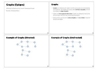
Graphs Graph G = ( V , E ) connected components: transitive closure of “connectivity relation” 4 / 15

Graphs Graph G = ( V , E ) connected components: transitive closure of “connectivity relation” diameter: longest among all pairwise shortest paths (within components) 4 / 15

Graphs Graph G = ( V , E ) connected components: transitive closure of “connectivity relation” diameter: longest among all pairwise shortest paths (within components) Random graphs: N vertices, each edge tentative ( ij ) with prob. p . Erdös-Rényi: ( ij ) ∈ N ( 2 ) , p = c / N → finite connect. c two-dim. percolation: ( ij ) ∈ square lattice, p = const N vertices, given (sampled) degree sequence k 1 . . . . , k i , e.g., scale-free P ( k ) ∼ k − γ each graph with same probability (“configuration model”) 4 / 15

Physics Approach Idea: ↔ model physical system degrees of freedom � quenched realisation ↔ x (state) energy E ( � quantity “score” S ↔ x ) (ground state: often known) simulate at finite T Monte Carlo moves: change realisat. a bit Simulation at different T 20 (using (MC) 3 /PT) T=0.5 15 T=0.57 Example (sequence alignment) S(t) 10 T=0.69 equilibration: T=0.98 start with ground state/ 5 with random state 0 Wang-Landau approach 0 5000 10000 15000 20000 t 5 / 15

Distribution of Scores 0 10 Raw result − → −1 (simple ↔ T = ∞ ) 10 at low T : −2 10 high scores prefered * (S) p simple −3 10 MC moves: � x → � x ′ T=0.69 T=0.57 change on “element” −4 10 probability = f a −5 10 0 5 10 15 20 S Pr(acceptance) = min { 1 , exp ( S ( � x ′ ) / T ) x ) / T ) } = min { 1 , e ∆ S / T } exp ( S ( � x ) e S ( � x ) / T / Z ( T ) ⇒ equilibrium distribution Q T ( � x ) = P ( � x ) e S ( � with P ( � x P ( � x ) / T x ) = � i f x i , Z ( T ) = � � x ) = exp ( S / T ) x )= S Q T ( � x )= S P ( � ⇒ p T ( S ) = � � x ) � x , S ( � � x , S ( � Z ( T ) p ( S ) = p T ( S ) Z ( T ) e − S / T ⇒ [AKH, PRE 2001] 6 / 15

Match Distriutions � � p ( S ) = p T ( S ) Z ( T ) exp ( − S / T ) rescaling with exp ( − S / T ) Z ( T ) by “matching” 2 2 10 10 0 10 0 10 -2 10 p T (S) exp( -S/T) -2 -4 10 10 p(S) -6 10 -4 9 10 simple, N=10 -8 10 4 simple, N=10 simple -10 -6 T=0.69 10 10 T=0.69 T=0.57 T=0.57 -12 10 -8 10 0 10 20 0 10 20 S S agrees with large statistics simple sampling agrees with (for this example) known exact result 7 / 15

Results: Erd˝ os-Rényi Size S of largest component (connectivity c ) [AKH, Eur. Phys. J. B (2011)] 8 / 15

Rate function Φ( s ) ≡ − 1 N log P ( s ) , s = S / N Comparison with exact asymptotic result [M. Biskup, L. Chayes, S.A. Smith, Rand. Struct. Alg. 2007] → evaluate algorithm → works very well → finite-size corrections visible 9 / 15

Phase transition Cluster size as function of (artificial) temperature 1st order transition in percolating phase → large system sizes not fully accessible ( → use Wang-Landau algorithm here) 10 / 15

Bias in Configuration model Configuration model: k “stubs” for each node of degree k . Randomly draw pairs of stubs. If multiple/self edge: refusal: start graph from scratch repetition: redraw pair Repetition is biased: relevant for measurements ( N → ∞ ) ? γ = 2.5 n=8 20 11000 refusal repetition 15 No. graphs diameter 10000 10 5 refusal repetition refusal with cutoff repetition with cutoff 9000 0 0 100 200 300 400 10 50 100 200 realization n [H. Klein-Hennig, AKH, Phys. Rev. E 2012] → Markov chains/ hidden variables/ throw-away edges/ ... 11 / 15

Two-dimensional percolation N = L × L , edge density p No exact result known (to me) Results comparable to Erd˝ os-Rényi random graphs but stronger finite-size effects 12 / 15

Graph Diameter Diameter d ⋆ := Longest of all shortest i → j paths Random graphs: ( c < 1): Gumbel distribution Pr G ( d ⋆ = d ) = λ e − λ ( d − d 0 ) e − e − λ ( d − d 0 ) 0 10 (sloppy) explanation: graph = forest -5 10 d = max trees T d ( T ) -10 10 c=0.9 → Gumbel distribution P(d) -15 Fit to 10 0.4 -20 0.3 P ( d ) = P G ( d ) e − a ( d − d 0 ) 2 10 λ( N) N=100 0.2 N=200 -25 N=1000 10 N=5000 0.1 “gaussianized” Gumbel 2 3 4 10 10 10 fits N -30 10 [AKH, M. Mézard, in preparation] 0 50 100 d 13 / 15

Close to c = 1, asymptotically Percolating region: more complex distributions λ ( c ) = − log c [T. Luczak, Rand.Struct.Alg., 1998] 0.0 3.0 N → ∞ -log( c) 2.5 2.0 -0.5 c=3.0 φ (d/N) λ( c) 1.5 N=100 N=200 1.0 N=500 -1.0 N=1000 0.5 0.0 0 0.2 0.4 0.6 0.8 1 0 0.2 0.4 0.6 0.8 1 d/N c 14 / 15

Summary Large-deviation properties Physics approach: study system at artificial finite temperature (or, in principle, Wang-Landau algorithm + modifications) Full distribution of size of largest component Erd˝ os-Rényi random graphs: matches well analytics 1st order transition in percolating phase (also: number of components, 2d percolation, diameter) Simple sampling of configuration model is biased Work more efficiently: read/write/edit scientific paper summaries (open access) www.papercore.org Summer school: Efficient Algorithms in Computational Physics Bad Honnef (Germany), 10-14. September 2012 15 / 15