Language Models Fall 2020 2020-09-11 Adapted from slides from Anoop - PowerPoint PPT Presentation
SFU NatLangLab CMPT 413/825: Natural Language Processing Language Models Fall 2020 2020-09-11 Adapted from slides from Anoop Sarkar, Danqi Chen and Karthik Narasimhan 1 Announcements Sign up on Piazza for announcements, discussion, and
SFU NatLangLab CMPT 413/825: Natural Language Processing Language Models Fall 2020 2020-09-11 Adapted from slides from Anoop Sarkar, Danqi Chen and Karthik Narasimhan 1
Announcements • Sign up on Piazza for announcements, discussion, and course materials: piazza.com/sfu.ca/fall2020/cmpt413825 • Homework 0 is out — due 9/16, 11:59pm • Review problems on probability, linear algebra, and calculus • Programming - Setup group, github, and starter problem • Try to have unique group name • Make sure your Coursys group name and your GitHub repo name match • Avoid strange characters in your group name • Interactive Tutorial Session • 11:50am to 12:20pm - last 30 minutes of lecture • (optional) but recommended review of math background 2
Consider Today, in Vancouver, it is 76 F and red vs Today, in Vancouver, it is 76 F and sunny • Both are grammatical • But which is more likely? 3
Language Modeling • We want to be able to estimate the probability of a sequence of words • How likely is a given phrase / sentence / paragraph / document? Why is this useful? 4
Applications • Predicting words is important in many situations • Machine translation P (a smooth finish) > P (a flat finish) • Speech recognition/Spell checking P (high school principal ) > P (high school principle ) • Information extraction, Question answering 5
Language models are everywhere Autocomplete 6
Impact on downstream applications (Miki et al., 2006) 7
What is a language model? Probabilistic model of a sequence of words Setup : Assume a finite vocabulary of words V V = { killer , crazy , clown } can be used to construct a infinite set of sentences (sequences of words) V V + = { clown , killer clown , crazy clown , crazy killer clown , killer crazy clown , …} s ∈ V + where a sentence is defined as where s = { w 1 , …, w n } 8
What is a language model? Probabilistic model of a sequence of words Given a training data set of example sentences S = { s 1 , s 2 , …, s N }, s i ∈ V + Estimate a probability model p ( s i ) = ∑ ∑ p ( w 1 , …, w n i ) = 1.0 s i ∈ V + i Language Model 9
Learning language models How to estimate the probability of a sentence? • We can directly count using a training data set of sentences P ( w 1 , …, w n ) = c ( w 1 , …, w n ) • N is a function that counts how many times each sentence • c occurs • N is the sum over all possible values c ( ⋅ ) 10
Learning language models How to estimate the probability of a sentence? P ( w 1 , …, w n ) = c ( w 1 , …, w n ) N • Problem : does not generalize to new sentences unseen in the training data • What are the chances you will see a sentence crazy killer clown crazy killer • In NLP applications, we often need to assign non-zero probability to previously unseen sentences 11
Estimating joint probabilities with the chain rule p ( w 1 , w 2 , …, w n ) = p ( w 1 ) p ( w 2 | w 1 ) p ( w 3 | w 1 , w 2 ) × … × p ( w n | w 1 , w 2 , …, w n − 1 ) Example Sentence: “the cat sat on the mat” P (the cat sat on the mat) = P (the) ∗ P (cat | the) ∗ P (sat | the cat) ∗ P (on | the cat sat) ∗ P (the | the cat sat on) ∗ P (mat | the cat sat on the) 12
Estimating probabilities P (sat | the cat) = count(the cat sat) Maximum likelihood Let’s count count(the cat) estimate again! (MLE) P (on | the cat sat) = count(the cat sat on) count(the cat sat) • With a vocabulary of size | V | • # sequences of length : n | V | n • Typical vocabulary ~ 50k words • even sentences of length ≈ 4.9 × 10 51 results in sequences! ≤ 11 ≈ 10 50 (# of atoms in the earth ) 13
Markov assumption • Use only the recent past to predict the next word • Reduces the number of estimated parameters in exchange for modeling capacity • 1st order P (mat | the cat sat on the) ≈ P (mat | the) • 2nd order P (mat | the cat sat on the) ≈ P (mat | on the) 14
k th order Markov • Consider only the last k words for context which implies the probability of a sequence is: (k+1) gram 15
n-gram models n Y Unigram P ( w 1 , w 2 , ...w n ) = P ( w i ) i =1 n Y P ( w 1 , w 2 , ...w n ) = P ( w i | w i − 1 ) Bigram i =1 and Trigram, 4-gram, and so on. Larger the n, more accurate and better the language model (but also higher costs) Caveat: Assuming infinite data! 16
Unigram Model 17
Bigram Model 18
Trigram Model 19
Maximum Likelihood Estimate 20
Number of Parameters Question 21
Number of Parameters Question 22
Number of Parameters Question 23
Number of parameters 24
Generalization of n-grams • Not all n-grams will be observed in training data! • Test corpus might have some that have zero probability under our model • Training set: Google news • Test set: Shakespeare • P (a ff ray | voice doth us) = 0 P(test corpus) = 0 25
Sparsity in language Frequency 1 freq ∝ rank Zipf’s Law Rank • Long tail of infrequent words • Most finite-size corpora will have this problem. 26
Smoothing n-gram Models 27
Handling unknown words 28
Smoothing • Smoothing deals with events that have been observed zero or very few times • Handle sparsity by making sure all probabilities are non-zero in our model • Additive: Add a small amount to all probabilities • Interpolation: Use a combination of di ff erent n-grams • Discounting: Redistribute probability mass from observed n-grams to unobserved ones • Back-o ff : Use lower order n-grams if higher ones are too sparse 29
Smoothing intuition Taking from the rich and giving to the poor (Credits: Dan Klein) 30
Add-one (Laplace) smoothing • Simplest form of smoothing: Just add 1 to all counts and renormalize! • Max likelihood estimate for bigrams: • Let be the number of words in our vocabulary. Assign | V | count of 1 to unseen bigrams • After smoothing: 31
Add-one (Laplace) smoothing 32
Additive smoothing (Lidstone 1920, Jeffreys 1948) • Why add 1? 1 is an overestimate for unobserved events • Additive smoothing ( ): 0 < δ ≤ 1 • Also known as add-alpha (the symbol is used instead of ) α δ 33
Linear Interpolation (Jelinek-Mercer Smoothing) ˆ P ( w i | w i − 1 , w i − 2 ) = λ 1 P ( w i | w i − 1 , w i − 2 ) + λ 2 P ( w i | w i − 1 ) + λ 3 P ( w i ) X λ i = 1 i • Use a combination of models to estimate probability • Strong empirical performance 34
Linear Interpolation (Jelinek-Mercer Smoothing) 35
Linear Interpolation: Finding lambda 36
Next Week • More on language models • Using language models for generation • Evaluating language models • Text classification • Video lecture on levels of linguistic representation 37
Recommend
More recommend
Explore More Topics
Stay informed with curated content and fresh updates.
