LA 2019 lect.#4 on Linear equation systems ++ Lecture showed slides - PowerPoint PPT Presentation
LA 2019 lect.#4 on Linear equation systems ++ Lecture showed slides 1 13, and covered (handwritten notes, separate file) algorithm pp. 1518 and examples. Slides 14 and 19ff: additional examples! First: what do we have? Vectors:
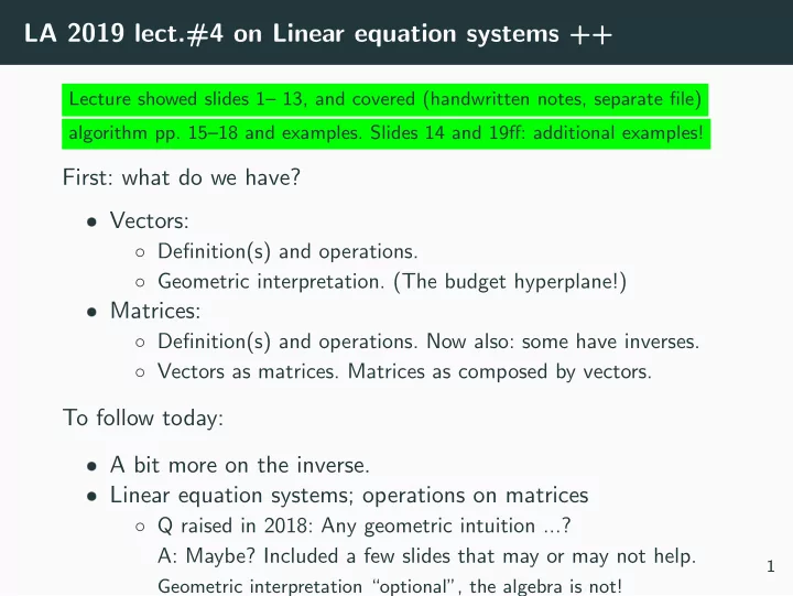
LA 2019 lect.#4 on Linear equation systems ++ Lecture showed slides 1– 13, and covered (handwritten notes, separate file) algorithm pp. 15–18 and examples. Slides 14 and 19ff: additional examples! First: what do we have? ❼ Vectors: ◦ Definition(s) and operations. ◦ Geometric interpretation. (The budget hyperplane!) ❼ Matrices: ◦ Definition(s) and operations. Now also: some have inverses. ◦ Vectors as matrices. Matrices as composed by vectors. To follow today: ❼ A bit more on the inverse. ❼ Linear equation systems; operations on matrices ◦ Q raised in 2018: Any geometric intuition ...? A: Maybe? Included a few slides that may or may not help. 1 Geometric interpretation “optional”, the algebra is not!
LA 2019 lect.#4: We defined the inverse First: the whole truth about the scalar equation αx = β , please! ❼ If α − 1 exists, then the only solution is α − 1 β . ❼ If there is no α − 1 : no solution unless β = 0, then all x solve. ❼ That “ α − 1 ” we often write 1 /α : we can divide by numbers. ❼ Matrices: cannot divide, but sometimes we have an “ A − 1 ” and can multiply. Definition: Given A . If there exists M such that MA = AM = I , then we call M the inverse of A and write A − 1 = M . ❼ A must necessarily be square. M must be of same order. ❼ Fact: A cannot have more than one inverse. ❼ Fact: If A is square, then you need only check one of AM = I or MA = I , because then the other holds automatically: For n × n matrices, AM = I holds if and only if MA = I 2 (Not at all obvious! True because n < ∞ ...)
LA 2019 lect.#4: n × n matrix: “left or right inverse” suffices Once we point out that A is square, we need only calculate one of the products. Examples: � − 1 � � � 1 − 2 4 − 2 Example: Show that = t for some t ∈ R . 3 − 4 3 − 1 � � � � � � 1 − 2 4 − 2 − 2 0 Solution: Multiply: t = t = − 2 t I . 3 − 4 3 − 1 0 − 2 True when t = − 1 / 2. � � � � 4 − 2 1 − 2 Or, just as good: reverse order. − 1 = I . 2 3 − 1 3 − 4 � − 1 � � � a b d − b 1 Example: If ad − bc � = 0, then = ad − bc c d − c a (Fact: If ad − bc = 0, then no inverse exists. � a b � For later: ad − bc is the determinant of .) 3 c d
LA 2019 lect.#4: n × n matrix: the inverse as solution to a linear equation system Once we point out that A is square ... cont’d: Fact: If A is square, then solving AX = I for X , yields X = A − 1 if it exists (and no solution if it doesn’t.) Why? Solving, we do get X such that AX = I iff that exists. Then we do not need to verify that XA = I . (Since A is square.) So once we can solve linear equation systems, you have one method for finding the inverse. Fact: If A is square, the following will hold true: Iff A − 1 exists, the equation system AX = B has unique solution X ; If so, this solution is X = A − 1 B . (The “ ⇐ = ” part requires A square. If not ... say, some equation repeats?) 4
LA 2019 lect.#4: Budget constraint as linear equation ❼ Suppose there are n goods in the economy, and you are about to choose x ∈ R n to consume 1 . ❼ The budget constraint p · x = β will remove one degree of freedom from your choice; if 2 p 1 � = 0, then once x 2 , . . . , x n are 1 � � chosen, x 1 will be pinned down to β − p 2 x 2 − · · · − p n x n . p 1 ❼ What if someone imposes another linear constraint r · x = γ on you? ◦ Next slide: n = 3; think of a budget ( 1, 3, 3 ) · ( x , y , z ) = 5 (the plane “with blue edge”!) and throw in another linear equation. 1 assuming you can actually consume negative amounts 2 what if p 1 = 0? Then choose some other non-free good to solve for. Works unless p = 0 ... in which case, what happens? 5
LA 2019 lect.#4: Linear equation systems visualized Visualization: assume n = 3. Two eq’s: 1 0 2 − 1 1 0 1 2 0 Two planes: ( 1, 0, 3 ) · ( x , y , z ) = 2 and ( 1, 3, 3 ) · ( x , y , z ) = 5. The intersection is the line ( x , y , z ) = ( 2, 1, 0 ) + t (− 3, 0, 1 ) . 6
LA 2019 lect.#4: Linear equation systems Requiring ( x , y , z ) to belong to (both simultaneously!) the two planes ( 1, 0, 3 ) · ( x , y , z ) = 2 and ( 1, 3, 3 ) · ( x , y , z ) = 5 and ( 1, 0, 3 ) · ( x , y , z ) = 2, is the same as imposing the system of two linear equations: x + 3 z = 2 & x + 3 y + 3 z = 5. � x � � � 1 0 3 2 Or, written on matrix form: y = 1 3 3 5 z ❼ Solution with one degree of freedom. (A line.) ❼ If there were another third equation: Would typically eliminate that degree of freedom and pin down one point where that third plane is hit by the line. ◦ ... but not necessarily so. E.g., if the third eq. is y = c : If c � = 1: impossible! If c = 1: still the same line. Next slide: general theory 7
LA 2019 lect.#4: Linear equation systems – theory A linear equation system for an unknown n × p matrix X is (or can be written as) AX = B where A is m × n , B is n × p ❼ Such an eq. system has either no solution, unique (i.e. precisely one) solution, or infinitely many solutions! ◦ If there are two distinct solutions, X and Y , then any Z = X + t ( Y − X ) also solves: AZ = AX + t ( AY − AX ) = B + t ( B − B ) , OK . ◦ If B = 0 m × p – a so-called homogeneous equation system – then there always is at least one solution, X = 0 n × p . ❼ Exam: You can be asked to “solve”. That means: Find all solutions, or show that none exists. ❼ Exam: You can be asked, e.g. “Does the equation system have zero, one or more than one solution?” That does not ask you to solve! ◦ System might depend on parameter c . Question type: “For what c ∈ R does the system A c x = b c have unique solution?” 8 (cont’d next slide)
LA 2019 lect.#4: Linear equation systems – theory / degrees of freedom Last sub-item had minuscle x and b c – i.e. column vectors, p = 1: ❼ Exam/syllabus: if p > 1, so X and B are not (column) vectors, then: ◦ You will not be asked to solve for infinitely many solutions. You will not be asked for degrees of freedom (see below). The rest of the previous slide you should know, though. Assume – for now – that p = 1, and consider Ax = b . Definition: Solution with d degrees of freedom means: d = 0: Unique solution. d ∈ N : Infinitely many solutions, such that there is some selection of d variables that can be chosen freely, and then, the n − d others are determined uniquely by the system. 9
LA 2019 lect.#4: Linear equation systems – vs scalar αx = β The case of one single equation in a single unknown? αx = β . ❼ Square coefficient matrix :-) ↔ as many equations as unknowns, cf. the counting rule – which is only a “rule of thumb”, not logically valid! ◦ If α − 1 exists (i.e. if α � = 0): Unique solution. ◦ If α − 1 does not exist: 0 x = β either has no solution (if β � = 0) or solution with one degree of freedom. What properties generalize from αx = β to AX = B , and how? ❼ A alone determines whether there is unique solution or not. ❼ If not unique: None or infinitely many; one must consider both A and B to determine (i) whether none or infinitely many; and (ii) if infinitely many: how many degrees of freedom. ❼ If A is square: unique solution iff A has an inverse M such that MA = I : more tomorrow! ❼ If A not square: start to solve! Math 2 has no other tools. 10
LA 2019 lect.#4: Linear equation systems – example Example: Back to x + 3 z = 2 & x + 3 y + 3 z = 5. Subtract eq’s to get 3 y = 3 and x + 3 z = 2, one degree of freedom: ❼ Either choose z = t ; then x will be given as y = 2 − 3 t ; ❼ Or, choose x = s ; then z will be given as z = ( 2 − s ) / 3. ❼ Note: y cannot be chosen freely. All solutions have y = 1. What did I just do to solve ... ? + 3 z = 2 + 3 z = 2 x ⇔ x − 1 x + 3 y + 3 z = 5 ← − 0 + 3 y + 0 = 3 + � � x x � � � � � � 1 0 3 2 1 0 3 2 Matrices: y = ⇔ y = 1 3 3 5 0 3 0 3 z z � � � � 1 0 3 | 2 1 0 3 | 2 Next up: write as ∼ . 1 3 3 | 5 0 1 0 | 1 11 (Scaled the last by 1/3, then it says “ y = 1”.)
LA 2019 lect.#4: Linear equation systems; more terminology. Lots of phrases coming up, some “not exam relevant 3 ”: Definition: The augmented coefficient matrix of the equation system AX = B , is the matrix ( A | B ) composed by stacking up B to the right of A . (Like on previous slide.) ❼ The | is not “completely standard” notation, but recommended to keep left-hand side from right-hand side. More terminology follows: 3 At the exam, you will not be asked “what is row-echelon form?” or “what are elementary row operations?” – what you need to, is do the work. But we need the language for teaching ... You will not be asked “what is Gaussian elimination?”, but you could be asked, e.g.: “Solve [...] by Gaussian elimination”, and then you must use that method – which means you must know which method it refers to. 12
Recommend
More recommend
Explore More Topics
Stay informed with curated content and fresh updates.
