L6: Multiparameter models example: Bioassay experiment Tuesday 14th - PDF document

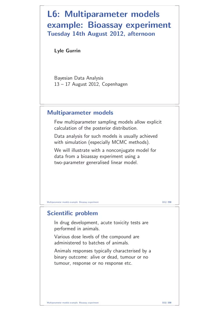
L6: Multiparameter models example: Bioassay experiment Tuesday 14th August 2012, afternoon Lyle Gurrin Bayesian Data Analysis 13 – 17 August 2012, Copenhagen Multiparameter models Few multiparameter sampling models allow explicit calculation of the posterior distribution. Data analysis for such models is usually achieved with simulation (especially MCMC methods). We will illustrate with a nonconjugate model for data from a bioassay experiment using a two-parameter generalised linear model. Multiparameter models example: Bioassay experiment 111/ 258 Scientific problem In drug development, acute toxicity tests are performed in animals. Various dose levels of the compound are administered to batches of animals. Animals responses typically characterised by a binary outcome: alive or dead, tumour or no tumour, response or no response etc. Multiparameter models example: Bioassay experiment 112/ 258

Data Structure Such an experiment gives rise to data of the form ( x i , n i , y i ); i = 1 , . . . , k (27) where x i is the i th dose level ( i = 1 , . . . , k ). n i animals given i th dose level. y i animals with positive outcome (tumour, death, response). Multiparameter models example: Bioassay experiment 113/ 258 Example Data For the example data, twenty animals were tested, five at each of four dose levels. Dose, x i Number of Number of (log g/ml) animals, n i deaths, y i − 0 . 863 5 0 − 0 . 296 5 1 − 0 . 053 5 3 0 . 727 5 5 Racine A, Grieve AP, Fluhler H, Smith AFM. (1986). Bayesian methods in practice: experiences in the pharmaceutical industry (with discussion). Applied Statistics 35 , 93-150. Multiparameter models example: Bioassay experiment 114/ 258 Sampling model at each dose level Within dosage level i : The animals are assumed to be exchangeable (there is no information to distinguish among them). We model the outcomes as independent given same probability of death θ i , which leads to the familiar binomial sampling model: y i | θ i ∼ Bin( n i , θ i ) (28) Multiparameter models example: Bioassay experiment 115/ 258

Setting up a model across dose levels Modelling the response at several dosage levels requires a relationship between the θ i ’s and x i ’s. We start by assuming that each θ i is an independent parameter. We relax this assumption tomorrow when we develop hierarchical models. There are many possibilities for relating the θ i ’s to the x i ’s, but a popular and reasonable choice is a logistic regression model: logit ( θ i ) = log( θ i / (1 − θ i )) = α + β x i (29) Multiparameter models example: Bioassay experiment 116/ 258 Setting up a model across dose levels We present an analysis based on a prior distribution for ( α , β ) that is independent and locally uniform in the two parameters, that is, p ( α , β ) ∝ 1 , so an improper “noninformative” distribution. We need to check that the posterior distribution is proper (details not shown). Multiparameter models example: Bioassay experiment 117/ 258 Describing the posterior distribution The form of posterior distribution: p ( α , β | y ) ∝ p ( α , β ) p ( y | α , β ) k � y i � � n i − y i e α + β x i � 1 � ∝ 1 + e α + β x i 1 + e α + β x i i =1 One approach would be to use a normal approximation centered at posterior mode α = 0 . 87 , ˜ (˜ β = 7 . 91) This is similar to the classical approach of obtaining maximum likelihood estimates ( eg by running glm in R ) Asymptotic standard errors can be obtained via ML theory. Multiparameter models example: Bioassay experiment 118/ 258

Bioassay graph 2 Contour plot: Posterior density of the parameters 30 25 20 beta 15 10 5 0 − 2 0 2 4 6 Multiparameter models example: Bioassay experiment 119/ 258 alpha Discrete approx. to the post. density (1) We illustrate computing the joint posterior distribution for ( α , β ) at a grid of points in 2-dimensions: 1. We begin with a rough estimate of the parameters. ◮ Since logit (E( y i /n i )) = α + β x i we obtain rough estimates of α and β using a linear regression of logit ( y i /n i ) on x i ◮ Set y 1 = 0 . 5 , y 4 = 4 . 5 to enable calculation. α = 0 . 1 , ˆ ◮ ˆ β = 2 . 9 (standard errors 0.3 and 0.5). Multiparameter models example: Bioassay experiment 120/ 258 Discrete approx. to the post. density (2) 2. Evaluate the posterior on a 200 × 200 grid; use range [ − 5 , 10] × [ − 10 , 40] . 3. Use R to produce a contour plot (lines of equal posterior density). 4. Renormalize on grid so � � β p ( α , β | y ) = 1 α (i.e., create discrete approx to posterior) 5. Sample from marginal dist’n of one parameter p ( α | y ) = � β p ( α , β | y ) . Multiparameter models example: Bioassay experiment 121/ 258

Discrete approx. to the post. density (3) 6. Sample from conditional dist’n of second parameter p ( β | α , y ) 7. We can improve sampling slightly by drawing from linear interpolation between grid points. Alternative: exact posterior using advanced computation (methods covered later) Multiparameter models example: Bioassay experiment 122/ 258 Posterior inference Quantities of interest: ◮ parameters ( α , β ) . ◮ LD50 = dose at which Pr( death ) is 0 . 5 = − α / β – This is meaningless if β ≤ 0 (substance not harmful). – We perform inference in two steps: (i) Pr ( β > 0 | y ) (ii) posterior dist’n of LD50 conditional on β > 0 Multiparameter models example: Bioassay experiment 123/ 258 Results We take 1000 simulation draws of ( α , β ) from the grid (di ff erent posterior sample than results in book) Note that β > 0 for all 1000 draws. Summary of posterior distribution posterior quantiles 2 . 5% 25% 50% 75% 97 . 5% α − 0 . 6 0 . 6 1 . 3 2 . 0 4 . 1 3 . 5 7 . 5 11 . 0 15 . 2 26 . 0 β LD 50 − 0 . 28 − 0 . 16 − 0 . 11 − 0 . 06 0 . 12 Multiparameter models example: Bioassay experiment 124/ 258

Lessons from simple examples The lack of multiparameter models with explicit posterior distributions not necessarily a barrier to analysis. We can use simulation, maybe after replacing sophisticated models with hierarchical or conditional models (possibly invoking a normal approximation in some cases). Multiparameter models example: Bioassay experiment 125/ 258 The four steps of Bayesian inference 1. Write the likelihood p ( y | θ ) . 2. Generate the posterior as p ( θ | y ) = p ( θ ) p ( y | θ ) by including well formulated information in p ( θ ) or else use p ( θ ) = constant. 3. Get crude estimates for θ as a starting point or for comparison. 4. Draw simulations θ 1 , θ 2 , . . . , θ L (summaries for y K for y 1 , ˜ y 2 , . . . . ˜ inference) and predictions ˜ each θ l . Multiparameter models example: Bioassay experiment 126/ 258