L. Li (LMD/CNRS): Three cells page 1 Zonally-averaged transport - PowerPoint PPT Presentation

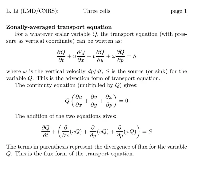
L. Li (LMD/CNRS): Three cells page 1 Zonally-averaged transport equation For a whatever scalar variable Q , the transport equation (with pres- sure as vertical coordinate) can be written as: ∂Q ∂t + u∂Q ∂x + v ∂Q ∂y + ω ∂Q ∂p = S where ω is the vertical velocity dp/dt , S is the source (or sink) for the variable Q . This is the advection form of transport equation. The continuity equation (multiplied by Q ) gives: � ∂u � ∂x + ∂v ∂y + ∂ω Q = 0 ∂p The addition of the two equations gives: � ∂ ∂Q ∂x ( uQ ) + ∂ ∂y ( vQ ) + ∂ � ∂t + ∂p ( ωQ ) = S The terms in parenthesis represent the divergence of flux for the variable Q . This is the flux form of the transport equation.

L. Li (LMD/CNRS): Three cells page 2 We can now apply the zonal average operator: ∂ [ Q ] + ∂ [ vQ ] + ∂ [ ωQ ] = [ S ] ∂t ∂y ∂p With the relationship [ vQ ] = [ v ][ Q ] + [ v ⋆ Q ⋆ ] , we obtain: ∂ [ Q ] + ∂ ∂y ([ v ][ Q ]) + ∂ ∂y ([ v ⋆ Q ⋆ ]) + ∂ ∂p ([ ω ][ Q ]) + ∂ ∂p ([ ω ⋆ Q ⋆ ]) = [ S ] ∂t One can use the continuity equation ∂ [ v ] ∂y + ∂ [ ω ] ∂p = 0 to write the transport equation as: � ∂ � � � ∂ [ Q ] [ v ] ∂ [ Q ] ∂y + [ ω ] ∂ [ Q ] ∂y ([ v ⋆ Q ⋆ ]) + ∂ ∂p ([ ω ⋆ Q ⋆ ]) + + = [ S ] ∂t ∂p Terms in the first parenthesis represent the advection of the mean circu- lation. Terms in the second parenthesis represent the divergence of eddy fluxes.

L. Li (LMD/CNRS): Three cells page 3 Zonally-averaged meridional circulation equation By using two basic equations, one is dynamic and another thermo- dynamic, we can deduce the equation that governs the meridional circu- lation: du dt − fv + ∂ Φ ∂x = F x dT dt − RT C p pω = J C p They can be changed to: � ∂ � � � ∂ [ u ] [ v ] ∂ [ u ] ∂y + [ ω ] ∂ [ u ] ∂y ([ v ⋆ u ⋆ ]) + ∂ ∂p ([ ω ⋆ u ⋆ ]) ∂t + + = f [ v ] + [ F x ] ∂p � ∂ ∂ [ T ] � [ v ] ∂ [ T ] ∂y + [ ω ] ∂ [ T ] � ∂y ([ v ⋆ T ⋆ ]) + ∂ � = RT C p p [ ω ]+[ J ] ∂p ([ ω ⋆ T ⋆ ]) ∂t + + ∂p C p

L. Li (LMD/CNRS): Three cells page 4 We need the following relationships (through scale analysis) to sim- plify furthermore the basic equations: [ ω ] ∂ [ u ] ∂p ≪ [ v ] ∂ [ u ] ∂y ∂ [ ω ⋆ u ⋆ ] ≪ ∂ [ v ⋆ u ⋆ ] ∂p ∂y ∂ [ u ] ∂y ≪ f Finally, we obtain: ∂t = f [ v ] − ∂ [ v ⋆ u ⋆ ] ∂ [ u ] + [ F x ] ∂y In the same manner, the thermodynamic equation can be transformed to: � RT [ ω ] − ∂ [ v ⋆ T ⋆ ] ∂ [ T ] C p p − ∂ [ T ] � + [ J ] = ∂t ∂p ∂y C p

L. Li (LMD/CNRS): Three cells page 5 Meridional overturning circulation stream function We can observe that the mean meridional mass circulation is non- divergent in the meriodional plane. Thus it can be represented in terms of a meridional mass transport streamfunction ψ . [ v ] and [ ω ] can be calculated by: [ v ] ≡ ∂ψ ∂p ; [ ω ] ≡ − ∂ψ ∂y This satisfies the continuity equation. ∂ [ v ] ∂y + ∂ [ ω ] ∂p = 0 ψ maximum ψ minimum Eq Pole N

L. Li (LMD/CNRS): Three cells page 6 How to calculate the stream function Mass continuity for the meridional circulation is: ∂ [ v ] ∂y + ∂ [ ω ] ∂p = 0 where ω is the vertical wind dp/dt . We can now introduce the stream function ψ to have the following equations: g ∂ [ ψ ] [ v ] = 2 πa cos φ ∂p and − g ∂ [ ψ ] [ ω ] = 2 πa 2 cos φ ∂φ The stream function can be calculated from the [ v ] field. It is enough to integrate the first equation from the top of the atmosphere with ψ = 0 as boundary condition.

L. Li (LMD/CNRS): Three cells page 7 Meridional overturning circulation of the atmosphere

L. Li (LMD/CNRS): Three cells page 8 Meridional overturning circulation of the atmosphere

L. Li (LMD/CNRS): Three cells page 9 Thermal wind equation to establish a relationship between u and T At this point, we need to use the geostrophic approximation and hydrostatic approximation f [ u ] = − ∂ [Φ] ∂y ∂ [Φ] ∂p = R [ T ] p to deduce the thermal wind equation f ∂ [ u ] ∂p = R ∂ [ T ] p ∂y If we take the time derivative of the thermal wind equation, we have: f ∂ � ∂ [ u ] � = R ∂ � ∂ [ T ] � ∂p ∂t p ∂y ∂t

L. Li (LMD/CNRS): Three cells page 10 Equation governing ψ Replace the terms ∂ [ u ] /∂t and ∂ [ T ] /∂t by the above equations, we obtain a diagnostic elliptique equation that governs the meridional cir- culation: ∂y 2 = f ∂ 2 [ v ⋆ u ⋆ ] ∂ 2 [ v ⋆ T ⋆ ] f 2 ∂ 2 ψ ∂p 2 + σ ∂ 2 ψ − R − f ∂ [ F x ] + R ∂ [ J ] ∂y = S ∂p∂y p ∂y 2 ∂p C p p where σ is the static stability σ ≡ RT C p P − ∂ [ T ] ∂p

L. Li (LMD/CNRS): Three cells page 11 S < 0 maximum ψ Eq Pole N Schematic of the meridional stream function

L. Li (LMD/CNRS): Three cells page 12 If the values of ψ on the boundaries are known, one can numerically solve this elliptic equation. This equation is also useful to diagnose qual- itatively the mean meridional circulation. Since ψ must vanish on the boundaries, it can be represented by a double Fourier series in y and p . M N A m B n sin( mπ p ) sin( nπ y � � ψ = ) δ p δ y m =1 n =1 Hence, the elliptic operator on the left is approximately proportional to − ψ . The four terms on the right, considered as sources, represent eddy momentum flux, eddy heat flux, zonal drag force and diabatic heating. ψ ∝ − f ∂ 2 [ v ⋆ u ⋆ ] ∂ 2 [ v ⋆ T ⋆ ] ; R ; f ∂ [ F x ] ∂p ; − R ∂ [ J ] ∂p∂y p ∂y 2 C p p ∂y

L. Li (LMD/CNRS): Three cells page 13 ψ ∝ − f ∂ 2 [ v ⋆ u ⋆ ] ; ∂ 2 [ v ⋆ T ⋆ ] ; f ∂ [ F x ] ∂p ; − ∂ [ J ] ∂p∂y ∂y 2 ∂y du/dt = 0 du/dt < 0 heating cooling Eq Pole N Eq Pole N

L. Li (LMD/CNRS): Three cells page 14 ψ ∝ − f ∂ 2 [ v ⋆ u ⋆ ] ; ∂ 2 [ v ⋆ T ⋆ ] ; f ∂ [ F x ] ∂p ; − ∂ [ J ] ∂p∂y ∂y 2 ∂y [v*u*] [v*u*] [v*T*] > 0 > 0 < 0 d/dz > 0 Eq Pole N Eq Pole N