L. Li (LMD/CNRS): Decompositions page 1 Statistics of the - - PowerPoint PPT Presentation

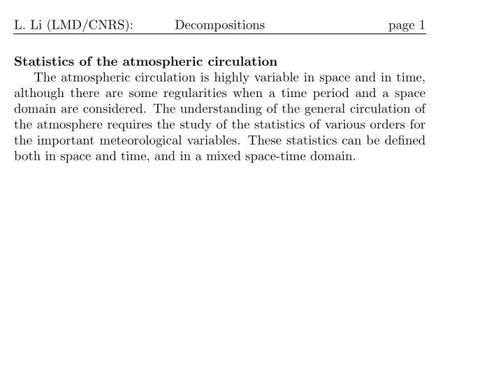
• L. Li (LMD/CNRS):

Decompositions page 1 Statistics of the atmospheric circulation The atmospheric circulation is highly variable in space and in time, although there are some regularities when a time period and a space domain are considered. The understanding of the general circulation of the atmosphere requires the study of the statistics of various orders for the important meteorological variables. These statistics can be defined both in space and time, and in a mixed space-time domain.

• L. Li (LMD/CNRS):

Decompositions page 2 Decomposition of the circulation into temporal mean and tran- sient eddies A represents a meteorological variable, such as temperature, humid- ity, winds, etc.), one can define the temporal mean m(A) = A = 1 τ τ Adt and the variance σ2(A) = 1 τ τ (A − A)2dt = 1 τ τ (A′)2dt A is the average and A′ is the deviation from the average. The instantaneous value of A is given by A = A + A′ Of course, A′ = 0. In practice, the variance σ2(A) can be calculated by the following

• L. Li (LMD/CNRS):

Decompositions page 3 equation which is easier for computation: σ2(A) = 1 τ τ A2dt − (1 τ τ Adt)2 = A2 − A

2

The average product of two quantities A and B is given by m(AB) = AB = (A + A′)(B + B′) = A B + A′B′ In this expression, the last term A′B′ is the covariance of A and B in time, and we define A′B′ = r(A, B)σ(A)σ(B) where r is the temporal correlation coefficient and σ the temporal stan- dard deviation. In practice, A′B′ is always obtained as a residual term: A′B′ = AB − A B If v is the meridional wind and q the specific humidity, then the meridional transport of water vapour can be written as: vq = v q + v′q′

• L. Li (LMD/CNRS):

Decompositions page 4 The left-side term is the total transport. It is decomposed into mean transport and transient-eddy transport. For kinetic energy which is the product of wind by itself, one can write: v2 = v2 + (v′)2 Total energy is thus decomposed into mean energy and transient energy.

• L. Li (LMD/CNRS):

Decompositions page 5 Decomposition of a variable into zonal mean and non-symmetric perturbation Fields such as wind velocity or temperature are also not uniform in space, varying both as a function of latitude and longitude. However meteorological conditions are generally more uniform along a latitude circle than in the north-south direction. It is thus convenient to define zonal-mean values at each latitude circle in order to assess the north- south variability. This can be achieved by introducing a zonal-average

• perator define by

[A] = 1 2π 2π Adλ and the departure from this average, A⋆, so that A = [A] + A⋆ Of course, [A⋆] = 0. The zonal average product of A and B is given by [AB] = [A][B] + [A⋆B⋆]

• L. Li (LMD/CNRS):

Decompositions page 6 In this expression, [A⋆B⋆]is the zonal or spatial covariance of A and B. If the two variables A and B fluctuate (in space) together, the covariance reaches its higest value. We can make a simple demonstration by using A⋆ = A0 sin(kx); B⋆ = B0 sin(kx + δ) where δ represent a phase difference between the two variables. A0 and B0 the amplitude (constant) of the two variables. One can show that [A⋆B⋆] = [A0B0 sin(kx) sin(kx + δ)] = A0B0 2 [cos(δ) − cos(2kx + δ)] = A0B0 2 cos(δ) It is clear that [A⋆B⋆] reaches its maximum value when δ = 0, that is, when the two variables oscillate in phase. This consideration is also applicable to the temporal transient variation. In the atmosphere, one can easily show that the non-symmetric circu- lation, due to the planetary waves, is in phase for v and T. This implies a positif heat transport to polar regions.

• L. Li (LMD/CNRS):

Decompositions page 7 Combination of temporal and spatial decompositions In a general manner, the temporal and spatial decompositions can be combined: A = [A] + A

⋆ + [A]′ + (A⋆)′

The term [A] represents the zonally symmetric part of the steady time- average quantity. The second term A

⋆ = [A] − [A] gives the asymmetric

part of the time-average quantity. The third term [A]′ = [A] − [A] rep- resents the instantaneous fluctuations of the symmetric part. The last term (A⋆)′ indicates the instantaneous, zonally asymmetric part. In practice, the zonal-mean decomposition is often realized after the temporal average: A = [A] + A

⋆

The last term represent the stationary perturbation. For the product of two variables: [AB] = [A B] + [A′B′] = [A][B] + [A

⋆B ⋆] + [A′B′]

The covariance of the two variables A and B is, in practice, always

• L. Li (LMD/CNRS):

Decompositions page 8

• btained as residual term:

[A

⋆B ⋆] = [A B] − [A][B]

If A is replaced by the meridional wind v, and B by the specific hu- midity q, one obtains then the equation governing the meridional trans- port of water vapour: [vq] = [v][q] + [v⋆q⋆] + [v′q′] The meridional transport of water vapour is thus decomposed into three terms, due to the mean circulation, stationary eddies and transient eddies respectively. If A and B are both replaced by the wind v, we obtain the kinetic energy decomposition: [v2] = [v]2 + [(v⋆)2] + [(v′)2]

• L. Li (LMD/CNRS):

Decompositions page 9 Various steps in diagnosing the atmospheric circulation Step 1: Calculate the temporal mean of the following quantities (3-D arrays for the three space dimensions): Simple terms: u, v, T, z, q Squared terms: u2, v2, T 2, z2, q2 Crossed terms: uv, uT, uz, uq, vT, vz, vq Additionals: e, ue, ve, θ, vθ, dθ/dp where e = CpT + Lq + gz + u2/2 + v2/2; θ = T(1000/p)R/Cp Step 2: Calculate the variance and covariance as residual terms by using the equation of their definition (3-D arrays for the three space dimensions). Variances: u′2, v′2, T ′2, z′2, q′2 Co-variances: u′v′, u′T ′, u′z′, u′q′, v′T ′, v′z′, v′q′ Step 3: Calculate the zonal averages (2-D arrays for two space dimen- sions Y-Z):

• For a simple quantity (q for example): [q], [q′2].
• For a crossed quantity (vq for example, water vapour meridional

• L. Li (LMD/CNRS):

Decompositions page 10 transport): – [vq] (total transport), – [v][q] (transport realized by the mean meridional circulation), – [v′q′] (transport realized by the transient eddies), – [v⋆q⋆] (transport realized by the stationary eddies), obtained as residual term: [v q] − [v][q]

• For a squared quantity (kinetic energy v2 for example). The de-

composition is similar as that for vq: total energy, energy in the zonal mean circulation, energy in the transient eddies and energy in the stationary eddies. Step 4: Make the vertical integration over the whole column of the atmosphere: Q = 1 g ps qdp Step 5: Calculate other diagnostics, such as the generalized E-P flux useful to understand the interaction between the mean flow and eddies.

• L. Li (LMD/CNRS):

Decompositions page 11 Zonally and annually averaged of Kinetic energy (u2 + v2)/2