L I K E L I H O O D F R E E I N F E R E N C E - PowerPoint PPT Presentation

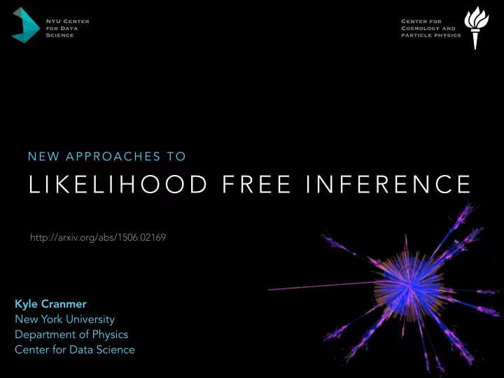
NYU Center Center for for Data Cosmology and Science particle physics N E W A P P R O A C H E S T O L I K E L I H O O D F R E E I N F E R E N C E http://arxiv.org/abs/1506.02169 Kyle Cranmer New York University Department of Physics Center for Data Science

P R E FA C E •This reminds me of PhyStat series leading up to the LHC. • Thanks to Louis, Tom, Bob, Richard, … • Impressed by the sophistication of discussion •One thing I learned: • collaboration might converge on high-level statistical procedure. Put in likelihood / probability model and turn the crank. • Practical improvements to analysis mainly lie in techniques used for modeling the data ! (eg. systematics, ND->FD extrapolation, etc.) • Useful to factorize discussion & software in terms of modeling and high-level statistical procedure 2

T H E H I G G S D I S C O V E RY " # n c Y Y Y f tot ( D sim , G| α ) = Pois( n c | ν c ( α )) f c ( x ce | α ) · f p ( a p | α p ) e =1 p ∈ S c ∈ channels 3

I N T R O D U C T I O N •In particle physics, our high-level inference goals are • searches (hypothesis testing) • measurements (maximum likelihood estimate) • constrain parameters (confidence intervals) •Typically, we use likelihood-based techniques • surprisingly, we lack a nice technique for likelihood- based inference when we want to use high-dimensional observations and have to deal with detector response 4

Likelihood-free Inference

O VERVIEW OF P REDICTIONS 1) The language is Quantum Field Theory Feynman Diagrams q 2) ν are used to predict W + l + W high-energy H interaction among - W W − l − fundamental particles ν ¯ q mu+ 3) The interaction of outgoing particles with the detector is simulated. e+ e- >100 million sensors 4) Finally, we run particle identification algorithms on the simulated data as if they were from real collisions. ~10-30 features describe interesting part mu- 6

D E T E C T O R S I M U L AT I O N • Conceptually: Prob(detector response | particles ) • Implementation: Monte Carlo integration over micro-physics •Consequence: cannot evaluate likelihood for a given event 7

D E T E C T O R S I M U L AT I O N • Conceptually: Prob(detector response | particles ) • Implementation: Monte Carlo integration over micro-physics •Consequence: cannot evaluate likelihood for a given event • This motivates a new class of algorithms for what is called likelihood-free inference , which only require ability to generate samples from the simulation in the “forward mode” 8

1 0 ⁸ S E N S O R S → 1 R E A L - VA L U E D Q U A N T I T Y •Most measurements and searches for new particles at the LHC are based on the distribution of a single variable or feature • choosing a good variable (feature engineering) is a task for a skilled physicist and tailored to the goal of measurement or new particle search • likelihood p(x| θ ) approximated using histograms (univariate density estimation) Events/10 GeV 40 ATLAS Preliminary Data 35 (*) Background ZZ Background Z+jets, t t 30 Signal (m =125 GeV) H Signal (m =190 GeV) H 25 Signal (m =360 GeV) H Syst.Unc. 20 (*) H ZZ 4l → → -1 ∫ s = 7 TeV: Ldt = 4.8 fb 15 -1 ∫ s = 8 TeV: Ldt = 5.8 fb 10 5 0 200 400 600 m [GeV] 4l This doesn’t scale if x is high dimensional! 9

H I G H D I M E N S I O N A L E X A M P L E •For instance, when looking for deviations from the standard model Higgs, we would like to look at all sorts of kinematic correlations • each observation x is high-dimensional 6000 6000 6000 6000 8000 8000 6000 6000 Events / ( 0.08 ) Events / ( 0.08 ) Events / ( 0.21 ) Events / ( 0.21 ) Events / ( 0.08 ) Events / ( 0.08 ) Events / ( 0.21 ) Events / ( 0.21 ) 4000 4000 6000 6000 4000 4000 4000 4000 4000 4000 2000 2000 2000 2000 2000 2000 2000 2000 0 0 0 0 0 0 0 0 -1 -1 -0.5 -0.5 0 0 0.5 0.5 1 1 -2 -2 0 0 2 2 -1 -1 -0.5 -0.5 0 0 0.5 0.5 1 1 -2 -2 0 0 2 2 cos cos θ θ * * Φ Φ cos cos θ θ or cos or cos θ θ Φ Φ 1 1 1 1 2 2 2000 2000 2000 2000 3000 3000 2000 2000 Events / ( 0.08 ) Events / ( 0.08 ) Events / ( 0.21 ) Events / ( 0.21 ) Events / ( 0.08 ) Events / ( 0.08 ) Events / ( 0.21 ) Events / ( 0.21 ) 1500 1500 1500 1500 2000 2000 1000 1000 1000 1000 1000 1000 1000 1000 500 500 500 500 0 0 0 0 0 0 0 0 -1 -1 -0.5 -0.5 0 0 0.5 0.5 1 1 -2 -2 0 0 2 2 -1 -1 -0.5 -0.5 0 0 0.5 0.5 1 1 -2 -2 0 0 2 2 cos cos θ θ * * Φ Φ cos cos θ θ or cos or cos θ θ Φ Φ 1 1 1 1 2 2 l 3000 3000 10000 10000 3000 3000 Events / ( 0.08 ) Events / ( 0.08 ) Events / ( 0.21 ) Events / ( 0.21 ) Events / ( 0.08 ) Events / ( 0.08 ) Events / ( 0.21 ) Events / ( 0.21 ) 4000 4000 2000 2000 2000 2000 l 5000 5000 2000 2000 1000 1000 1000 1000 H 0 0 0 0 0 0 0 0 -1 -1 -0.5 -0.5 0 0 0.5 0.5 1 1 -2 -2 0 0 2 2 -1 -1 -0.5 -0.5 0 0 0.5 0.5 1 1 -2 -2 0 0 2 2 cos cos * * cos cos or cos or cos θ θ Φ Φ θ θ θ θ Φ Φ 1 1 1 1 2 2 4000 4000 4000 4000 l 10000 10000 Events / ( 0.08 ) Events / ( 0.08 ) Events / ( 0.21 ) Events / ( 0.21 ) Events / ( 0.08 ) Events / ( 0.08 ) Events / ( 0.21 ) Events / ( 0.21 ) 3000 3000 3000 3000 4000 4000 2000 2000 2000 2000 5000 5000 l 2000 2000 1000 1000 1000 1000 0 0 0 0 0 0 0 0 -1 -1 -0.5 -0.5 0 0 0.5 0.5 1 1 -2 -2 0 0 2 2 -1 -1 -0.5 -0.5 0 0 0.5 0.5 1 1 -2 -2 0 0 2 2 cos cos θ θ * * Φ Φ cos cos θ θ or cos or cos θ θ Φ Φ 1 1 1 1 2 2 10

M O V I N G C L O S E R T O T H E D ATA •A more extreme example is to work with lower-level data • each observation x is high-dimensional LArTPC Pattern recognition with 2D ADC images in LArTPC P. Płoński, D. Stefan, R. Sulej Time Projection Chamber Electric Field Electric Field Electric Field Electric Field Electric Field Electric Field … informal input to the workshop discussions … γ γ ν µ γ γ γ γ γ γ DS@HEP Workshop, NYC, July 7, 2016 1 Neutrino interaction in LAr produces Drift the ionization charge in a Read out charge and light produced ionization and scintillation light uniform electric field using precision wires and PMT's ArgoNeuT Data ArgoNeuT Data ArgoNeuT Data ArgoNeuT Data Jonathon Asaadi candidate e candidate ν e ν CNNs Applied to MicroBooNE Vic Genty @ Columbia U. with MicroBooNE Deep Learning Team 
 Neutral Current Neutral Current G. Collins @ MIT candidate γ candidate K. Terao @ Columbia γ candidate 0 candidate π 0 π ArgoNeuT Data ArgoNeuT Data T. Wongjirad @ MIT MicroBooNE-NOTE-1019-PUB Convolutional Neural Networks Applied to Neutrino Tracking, Calorimetry, and Particle ID in same detector. Events in a Liquid Argon Time Projection Chamber Goal ~80% Neutrino Efficiency. MicroBooNE Collaboration July 4, 2016 All you need for Physics is neutrino flavor and energy. http://www-microboone.fnal.gov/publications/publicnotes/MICROBOONE-NOTE-1019-PUB.pdf 1 vgenty 11

L I K E L I H O O D F R E E I N F E R E N C E • Goal : approximate the likelihood p(x| θ ) for high dimensional feature x using a generative model for the data 7 ) H F ATLAS and CMS H m → γ γ f κ 2 ATLAS and CMS ( H ZZ 4 → → l Λ 6 LHC Run 1 LHC Run 1 Combined +4 l 2ln γ γ 1.5 Preliminary Stat. only uncert. − 5 H → γ γ 1 H ZZ → H WW → 4 0.5 H bb → H → τ τ 0 3 Combined 0.5 − 2 1 − 1 1.5 − SM 68% CL 2 − Best fit 95% CL 0 124 124.5 125 125.5 126 0 0.5 1 1.5 2 m [GeV] H f κ 12 V

L I K E L I H O O D F R E E I N F E R E N C E • Goal : approximate the likelihood p(x| θ ) for high dimensional feature x using a generative model for the data 1.5 excluded at CL > 0.95 excluded area has CL > 0.95 γ 1.0 ∆ m & ∆ m s d sin 2 β 0.5 m ∆ d ε α K γ β η 0.0 α V ub α -0.5 ε -1.0 K γ sol. w/ cos 2 β < 0 (excl. at CL > 0.95) -1.5 -1.0 -0.5 0.0 0.5 1.0 1.5 2.0 ρ Figure 11.2: Constraints on the ¯ ρ , ¯ η plane. The shaded areas have 95% CL. C 13

T H E R A P I D R I S E O F “ A B C ” 14

A N A LT E R N AT I V E T O A B C K.C., http://arxiv.org/abs/1506.02169

C O L L A B O R AT O R S Gilles Louppe Juan Pavez Data Science Fellow CS graduate student in Chile Funded via NSF DIANA/HEP Fellowship to work @ CERN summer ’15 Based at CERN @jgpavez PhD in machine learning scikit-learn developer @glouppe 16

M A C H I N E L E A R N I N G : C L A S S I F I E R S •Common to use machine learning classifiers to separate signal (H 1 ) vs. background (H 0 ) • want a function that maps signal to y=1 and background to y=0 • think of it as applied calculus of variations: find function s(x) that minimizes loss : Normalized Normalized Signal 1.8 1.8 Background 1.6 1.6 Z p ( x | H 0 ) (0 − s ( x )) 2 dx 1.4 1.4 L [ s ] = 1.2 1.2 U/O-flow (S,B): (0.0, 0.0)% / (0.0, 0.0)% 1 1 Z p ( x | H 1 ) (1 − s ( x )) 2 dx + 0.8 0.8 0.6 0.6 0.4 0.4 X ( y i − s ( x i )) 2 ≈ 0.2 0.2 0 0 i -0.8 -0.8 -0.6 -0.6 -0.4 -0.4 -0.2 -0.2 -0 -0 0.2 0.2 0.4 0.4 0.6 0.6 s 0.8 0.8 17 BDT BDT