Revisiting Frank-Wolfe Projection-Free Sparse Convex Optimization - PowerPoint PPT Presentation
Revisiting Frank-Wolfe Projection-Free Sparse Convex Optimization Martin Jaggi Ecole Polytechnique Smile in Paris Seminar 2013 / 01 / 24 [ Paper ] Constrained Convex Optimization D R d f ( x ) x D f ( x ) min x D R d f ( x ) x
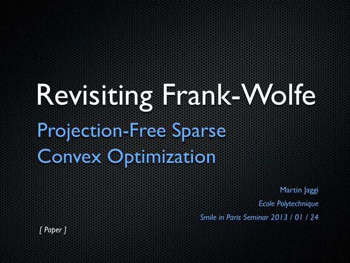
Revisiting Frank-Wolfe Projection-Free Sparse Convex Optimization Martin Jaggi Ecole Polytechnique Smile in Paris Seminar 2013 / 01 / 24 [ Paper ]
Constrained Convex Optimization D ⊂ R d
f ( x ) x ∈ D f ( x ) min x D ⊂ R d
f ( x ) x ∈ D f ( x ) min x D ⊂ R d
f ( x ) x ∈ D f ( x ) min x D ⊂ R d
f ( x ) x ∈ D f ( x ) min x D ⊂ R d
Frank-Wolfe Algorithm f ( x ) “Conditional Gradient Method” “Reduced Gradient Method” x D ⊂ R d AN ALGORITHM FOR QUADRATIC PROGRAMMING Marguerite Frank and P h i l i p Wolfel r Pr in c e t o n U n i v e r s i t y A finite iteration method for calculating the solution of quadratic programming problems is described. 1956 linear Droblems a r e suggested. Extensions to more general non- 1 . INTRODUCTION The problem of maximizing a concave quadratic function whose variables are subject to linear inequality constraints has been the subject of several recent studies, from both the com- putational side and the theoretical method for solving this non-linear programming problem which should be particularly well adapted to high-speed machine computation. ( s e e Bibliography). Our aim The quadratic programming problem as such, called PI, is set forth in Section 2. h e r e has been to develop a We find in Section 3 that with the aid of generalized Lagrange multipliers the'solutions of PI can be exhibited in a simple way as parts of the solutions of a new quadratic programming problem, called PII, which embraces the multipliers. The maximum sought in PI1 is known to be zero. A test for the existence of solutions to PI arises from the fact that the boundedness of i t s objective function i s In Section 4 we apply to PII an iterative process in which the principal computation is equivalent to the simplex method change-of-basis. One step of our "gradient and interpolation" method, t h e feasibility of given an initial feasible point, selects by the simplex routine a secondary basic feasible point t h e (linear) constraints of PII. whose projection along the gradient of the objective function at the initial point is sufficiently large. The point at which the objective is maximized for the segment joining the initial and secondary points is then chosen as the initial point for the next step. The values of the objective function on the initial points thus obtained converge to zero; but a remarkable feature of the quadratic problem is that in some step a secondary point which is a solution of the problem will be found, insuring the termination of A simplex technique machine program requires little alteration for the employment of this method. Limited experience suggests that solving a quadratic program in n variables and m constraints will take about as long as solving a linear program having m + n constraints and a "reasonable" number t h e process. Section 5 o f variables. of generalized Lagrange multipliers. discusses, for completeness, some other computational proposals making use Section 6 carries over the applicable part of the method, the gradient-and-interpolation routine, to the maximization of an arbitrary concave function under linear constraints (with one qualification). Convergence to the maximum is obtained as above, but termination of the process in an exact solution is not, although an estimate of error is readily found. In Section '7 (the Appendix) are accumulated some facts about linear programs and con- cave functions which are used throughout the paper. lUnder contract with the Office of Naval Research. 95
f ( x ) The Linearized Problem s 0 � x , r f ( x ) ⌦ ↵ s 0 2 D f ( x ) + min x s D ⊂ R d Algorithm 1 Frank-Wolfe Let x (0) 2 D for k = 0 . . . K do s 0 , r f ( x ( k ) ) ⌦ ↵ Compute s := arg min s 0 2 D 2 Let γ := k +2 Update x ( k +1) := (1 � γ ) x ( k ) + γ s end for
f ( x ) The Linearized Problem s 0 � x , r f ( x ) ⌦ ↵ s 0 2 D f ( x ) + min x D ⊂ R d r f ( x ) Frank-Wolfe Gradient Descent (approx.) solve Cost per step Projection back to D linearized problem on D ✓ ✗ Sparse Solutions (in terms of used vertices)
Algorithm Variants Line-Search Algorithm 1 Frank-Wolfe Algorithm 2 Frank-Wolfe for k = 0 . . . K do for k = 0 . . . K do s 0 , r f ( x ( k ) ) ⌦ ↵ s 0 , r f ( x ( k ) ) Compute s := arg min ⌦ ↵ Compute s := arg min s 0 2 D s 0 2 D 2 Let γ := Optimize γ by line-search k +2 Update x ( k +1) := (1 � γ ) x ( k ) + γ s Update x ( k +1) := (1 � γ ) x ( k ) + γ s end for end for Fully Corrective Algorithm 3 Frank-Wolfe for k = 0 . . . K do s 0 , r f ( x ( k ) ) ⌦ ↵ Compute s := arg min • Approximate s 0 2 D Update x ( k +1) := arg min f ( x ) x 2 conv( s (0) ,..., s ( k +1) ) Subproblems end for [ Dunn et al. 1978 ] • Away-Steps [ GuéLat et al. 1986 ]
What’s new? • Primal-Dual Analysis (and certificates for approximation quality) • Approximate Subproblems (and domains) • Affine Invariance • Optimality in Terms of Sparsity • More Applications
Convergence Analysis Primal Convergence: Primal-Dual Convergence: Algorithms obtain Algorithms obtain � 1 � 1 gap ( x ( k ) ) ≤ O � f ( x ( k ) ) − f ( x ∗ ) ≤ O � k k after steps . after steps . k k [ Frank & Wolfe 1956 ] [ Clarkson 2008, J. 2013 ]
A Simple Optimization Duality Original Problem x ∈ D f ( x ) min f ( x ) The Dual Value gap (x) ω ( x ) := s 0 � x , r f ( x ) ⌦ ↵ s 0 2 D f ( x ) + min ω ( x ) Weak Duality x D ⊂ R d ω ( x ) ≤ f ( x ⇤ ) ≤ f ( x 0 )
min x ∈ D f ( x ) Affine Invariance r f ( x ) x r f ( x ) x s s D ⊂ R d D ⊂ R d
Optimization over Atomic Sets min x ∈ D f ( x ) convex hull of things atoms A D := conv ( A ) Fact: Any linear function will attain its minimum over at an atom s ∈ A D [ Chandrasekaran et al. 2012 ]
Sparse Approximation x ∈ ∆ n f ( x ) min D := conv ( { e i | i ∈ [ n ] } ) unit simplex Corollary: � 1 � Obtain -approximate O k k solution of sparsity . lower bound: � 1 [ Clarkson 2008 ] � Ω Trade-Off: k Approximation quality vs sparsity f ( x ) := k x k 2 2
k D x � y k 2 Sparse Approximation 2 k x k 1 1 f ( x ) min D := conv ( {± e i | i ∈ [ n ] } ) ` 1 -ball Corollary: � 1 � Obtain -approximate O k k solution of sparsity . lower bound: � 1 � Ω Trade-Off: k Approximation quality vs sparsity Greedy Algorithms in Signal Processing: Equivalent to (Orthogonal) Matching Pursuit
Low Rank Approximation k X k ∗ 1 f ( X ) min uv T � ⇣n o⌘ u 2 R n , k u k 2 =1 D := conv � v 2 R m , k v k 2 =1 � trace-norm-ball Corollary: � 1 � Obtain -approximate O k solution of rank . k lower bound: � 1 � Ω Trade-Off: k Approximation quality vs rank Projection: FW-step: Requires full SVD approx. top singular vector [ J. & Sulovsk ý 2010 ]
- norm problems ` p k x k p 1 f ( x ) min -ball ` p D := p=4 Projection: FW-step: unknown? linear time p=1. 3
Examples of Atomic Domains Suitable for Frank-Wolfe X Optimization Domain Complexity of one Frank-Wolfe Iteration Atoms A D = conv( A ) sup s 2 D h s , y i Complexity R n Sparse Vectors k . k 1 -ball k y k 1 O ( n ) R n Sign-Vectors k . k 1 -ball k y k 1 O ( n ) R n ` p -Sphere k . k p -ball k y k q O ( n ) R n Sparse Non-neg. Vectors Simplex ∆ n max i { y i } O ( n ) � ⇤ � � R n P Latent Group Sparse Vec. k . k G -ball max g 2 G g 2 G | g | � y ( g ) g p ˜ R m ⇥ n � " 0 � Matrix Trace Norm k . k tr -ball k y k op = � 1 ( y ) O N f / (Lanczos) R m ⇥ n Matrix Operator Norm k . k op -ball k y k tr = k ( � i ( y )) k 1 SVD R m ⇥ n Schatten Matrix Norms k ( � i ( . )) k p -ball k ( � i ( y )) k q SVD ˜ f ( n + m ) 1 . 5 / " 0 2 . 5 � R m ⇥ n � Matrix Max-Norm k . k max -ball O N O ( n 3 ) R n ⇥ n Permutation Matrices Birkho ff polytope R n ⇥ n Rotation Matrices SVD (Procrustes prob.) p ˜ S n ⇥ n Rank-1 PSD matrices � " 0 � � max ( y ) O N f / (Lanczos) { x ⌫ 0 , Tr( x )=1 } of unit trace ˜ PSD matrices f n 1 . 5 / " 0 2 . 5 � S n ⇥ n � O N { x ⌫ 0 , x ii 1 } of bounded diagonal Table 1: Some examples of atomic domains suitable for optimization using the Frank-Wolfe algorithm. Here SVD refers to the complexity of computing a singular value decomposition, which is O (min { mn 2 , m 2 n } ) . N f is the number of non-zero entries in the gradient of the objective func- tion f , and " 0 = 2 δ C f k +2 is the required accuracy for the linear subproblems. For any p 2 [1 , 1 ] , the conjugate value q is meant to satisfy 1 p + 1 q = 1 , allowing q = 1 for p = 1 and vice versa. [J. 2013]
Recommend
More recommend
Explore More Topics
Stay informed with curated content and fresh updates.


