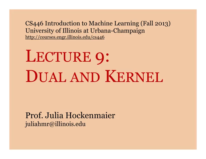
L ECTURE 9: D UAL AND K ERNEL Prof. Julia Hockenmaier - - PowerPoint PPT Presentation

CS446 Introduction to Machine Learning (Fall 2013) University of Illinois at Urbana-Champaign

http://courses.engr.illinois.edu/cs446

• Prof. Julia Hockenmaier

juliahmr@illinois.edu

LECTURE 9: DUAL AND KERNEL

CS446 Machine Learning

Linear classifiers so far…

What we’ve seen so far is not the whole story – We’ve assumed that the data are linearly separable – We’ve ignored the fact that the perceptron just finds some decision boundary, but not necessarily an optimal decision boundary

2

CS446 Machine Learning

Data are not linearly separability

3

Noise / outliers Target function is not linear in X

CS446 Machine Learning

Dual representation

• f linear classifiers

4

CS446 Machine Learning

Dual representation

Recall the Perceptron update rule: If xm is misclassified, add ym·xm to w if ym·f(xm) = ym·w·xm < 0:

w := w + ym·xm

Dual representation: Write w as a weighted sum of training items: w = ∑n αn yn xn αn: how often was xn misclassified? f(x) = w·x = ∑n αn yn xn ·x

5

CS446 Machine Learning

Dual representation

Primal Perceptron update rule: If xm is misclassified, add ym·xm to w if ym·f(xm) = ym·w·xm < 0:

w := w + ym·xm

Dual Perceptron update rule: If xm is misclassified, add 1 to αm if ym· ∑d αdxd·xm < 0:

αm

:= αm + 1

6

CS446 Machine Learning

Dual representation

Classifying x in the primal: f(x) = w x w = feature weights (to be learned) wx = dot product between w and x Classifying x in the dual: f(x) = ∑n αn yn xn x αn = weight of n-th training example (to be learned) xn x = dot product between xn and x The dual representation is advantageous when #training examples ≪ #features (requires fewer parameters to learn)

7

Kernels

CS446 Machine Learning

Making data linearly separable

9

• 2
• 1.5
• 1
• 0.5

0.5 1 1.5 2

• 2
• 1.5
• 1
• 0.5

0.5 1 1.5 2 x2 x1 Original feature space

f(x) = 1 iff x1

2 + x2 2 ≤ 1

0.5 1 1.5 2 0.5 1 1.5 2 x2*x2 x1*x1 Transformed feature space

CS446 Machine Learning

Making data linearly separable

10

Transform data: x = (x1, x2

) => x’ = (x1 2, x2 2 )

f(x’) = 1 iff x’1 + x’2 ≤ 1

CS446 Machine Learning

Making data linearly separable

These data aren’t linearly separable in the x1 space But adding a second dimension with x2 = x1

2

makes them linearly separable in 〈x1, x2〉:

11

x1 x1 x1

2

CS446 Machine Learning

Making data linearly separable

It is common for data to be not linearly separable in the original feature space. We can often introduce new features to make the data linearly separable in the new space: – transform the original features (e.g. x → x2) – include transformed features in addition to the original features – capture interactions between features (e.g. x3 = x1x2) But this may blow up the number of features

12

CS446 Machine Learning

Making data linearly separable

We need to introduce a lot of new features to learn the target function. Problem for the primal representation: w now has a lot of elements, and we might not have enough data to learn w The dual representation is not affected

13

CS446 Machine Learning

The kernel trick

– Define a feature function φ(x) which maps items x into a higher-dimensional space. – The kernel function K(xi, xj) computes the inner product between the φ(xi) and φ(xj) K(xi, xj) = φ(xi)φ(xj) – Dual representation: We don’t need to learn w in this higher-dimensional space. It is sufficient to evaluate K(xi, xj)

14

CS446 Machine Learning

Quadratic kernel

Original features: x = (a, b) Transformed features: φ(x) = (a2, b2, √2·ab) Dot product in transformed space: φ(x1)·φ(x2) = a1

2a2 2 + b1 2b2 2, 2·a1b1a2b2

= (x1·x2)2 Kernel: K(x1, x2) = (x1·x2)2 = φ(x1)·φ(x2)

15

CS446 Machine Learning

Polynomial kernels

Polynomial kernel of degree p: – Basic form K(xi,xj) = (xi ·xj)p – Standard form (captures all lower order terms): K(xi,xj) = (xi ·xj + 1)p

16

CS446 Machine Learning

From dual to kernel perceptron

Dual Perceptron: f(x) = ∑d αd xd·xm

Update: If xm is misclassified, add 1 to αm

if ym· ∑d αd xd·xm < 0:

αm

:= αm + 1

Kernel Perceptron: f(x) = ∑d αd φ(xd)·φ(xm) = ∑d αd K(xd·xm)

Update: If xm is misclassified, add 1 to αm

if ym· ∑d αd K(xd·xm) < 0:

αm

:= αm + 1

17

Maximum margin classifiers

CS446 Machine Learning

Maximum margin classifiers

19

Hard vs. soft margins

CS446 Machine Learning

Dealing with outliers: Slack variables ξi

ξi measures by how much example (xi, yi) fails to achieve margin δ

21

CS446 Machine Learning

Soft margins

Minimize training error while maximizing the margin ∑i ξi is an upper bound on the number of training errors C controls tradeoff between margin and training error

22

min

w

1 2 w⋅w subject to y1(w⋅x1) ≥1 ... yn(w⋅xn) ≥1

Hard margin (primal)

min

w

1 2 w⋅w +C ξi

i=1 n

∑

subject to ξi ≥ 0 ∀i y1(w⋅x1) ≥ (1−ξ1) and ξ1 ≥ 0 ... yn(w⋅xn) ≥ (1−ξn) and ξn ≥ 0

Soft margin (primal)