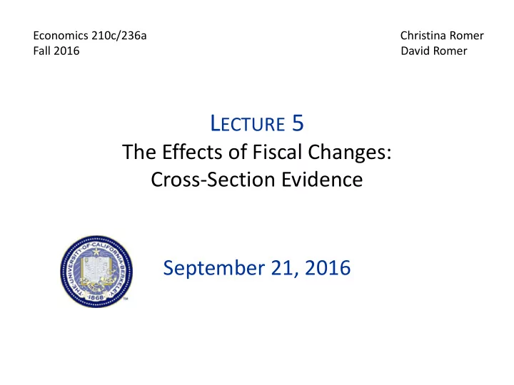
L ECTURE 5 The Effects of Fiscal Changes: Cross-Section Evidence - PowerPoint PPT Presentation
Economics 210c/236a Christina Romer Fall 2016 David
Economics 210c/236a Christina Romer Fall 2016 David Romer L ECTURE 5 The Effects of Fiscal Changes: Cross-Section Evidence September 21, 2016
I. O VERVIEW OF S TATE -B ASED S TUDIES OF THE I MPACT OF F ISCAL C HANGES
How does monetary policy affect the fiscal multiplier?
Open Economy Relative Multiplier • Multiplier: Effect of G on Y • Relative: How relative G in a state or region affects relative Y or employment • Open Economy: Are effects of spending in a state felt in the state?
How does the open economy relative multiplier compare with the closed economy aggregate multiplier? • Impact of monetary policy • State spillovers • Impact of Ricardian equivalence and crowding out
II. C HODOROW -R EICH , F EIVESON , L ISCOW , AND W OOLSTON , “D OES S TATE F ISCAL R ELIEF D URING R ECESSIONS I NCREASE E MPLOYMENT ? E VIDENCE FROM THE A MERICAN R ECOVERY AND R EINVESTMENT A CT ”
Experiment They Consider • ARRA increased aid to states to pay for Medicaid (FMAP). • Look at whether states that got more aid did better. • Main outcome variable is employment by state.
Omitted Variable Problem • More troubled states got more state fiscal relief in ARRA. • Solution: IV using 2007 state FMAP spending per person as instrument for ARRA FMAP increase. • Idea is that some states got more ARRA FMAP funds just because they had more generous systems before the recession.
C-R,F,L,W Specification Where: • E s is employment in state s • N s is the population aged 16+ in state s • AID s is state fiscal relief received by state s • Controls are state- and region-specific variables
From: Chodorow-Reich, Feiveson, Liscow, and Woolston
From: Chodorow-Reich, Feiveson, Liscow, and Woolston
Control Variables • Region dummies • Employment in manufacturing • Lagged state employment • Union share and Kerry vote share
From: Chodorow-Reich, Feiveson, Liscow, and Woolston
From: Chodorow-Reich, Feiveson, Liscow, and Woolston
From: Chodorow-Reich, Feiveson, Liscow, and Woolston
Timing of Impact • Do a Jordà-type procedure. • Run the cross-section regression many times, increasing the horizon by 1 month each time.
From: Chodorow-Reich, Feiveson, Liscow, and Woolston
From: Chodorow-Reich, Feiveson, Liscow, and Woolston
From: Chodorow-Reich, Feiveson, Liscow, and Woolston
Evaluation
III. N AKAMURA AND S TEINSSON , “F ISCAL S TIMULUS IN A M ONETARY U NION : E VIDENCE FROM U.S. R EGIONS ”
Experiment They Consider • Time series-cross section data on defense procurement by state. • Look at whether state GDP and employment respond to defense procurement by state.
From: Nakamura and Steinsson, “Fiscal Stimulus in a Monetary Union”
Omitted Variable Problem • State may be able to argue for more defense spending when local conditions are weak. • Could imagine OVB going the other way as well— states with successful military contractors are better at winning more contracts. • Going to use IV. • Key assumption: national defense spending is determined by geopolitical events, not local conditions.
IV Approach • Instruments are national defense spending as a share of GDP interacted with state dummy variables. • Variation comes from interaction of national shocks and differences in how sensitive state defense spending is to national spending. • Alternative variable (Bartik instrument) is G i /Y i in base period times G t /Y t .
From: Nakamura and Steinsson, “Fiscal Stimulus in a Monetary Union”
Nakamura and Steinsson’s Specification Where: Y it is output in state i in period t • G it is government procurement in state i in • period t α i are state fixed effects • γ t are year fixed effects •
How good are their instruments? • When use national defense interacted with state dummy, have 50 instruments. They tell us they have a weak instrument problem. • With Bartik instrument, only have one instrument. No weak instrument problem. • I would like to see more diagnostics on the first stage.
From: Nakamura and Steinsson, “Fiscal Stimulus in a Monetary Union”
From: Nakamura and Steinsson, “Fiscal Stimulus in a Monetary Union”
Nakamura and Steinsson’s Specification Where: Y it is output in state i in period t • G it is government procurement in state i in • period t α i are state fixed effects • γ t are year fixed effects • I it is an indicator for a period of low economic • slack
From: Nakamura and Steinsson, “Fiscal Stimulus in a Monetary Union”
Evaluation
Translating the Open-Economy Relative Multiplier into the Closed-Economy Aggregate Multiplier • Write down a complicated, optimizing model with two regions and calibrate it. • Generate data from the calibrated model based on different assumptions (such as sticky versus flexible prices, or accommodative versus counteracting monetary policy). • Estimate OERM and CEAM from the generated data to see how they compare.
From: Nakamura and Steinsson, “Fiscal Stimulus in a Monetary Union”
From: Nakamura and Steinsson, “Fiscal Stimulus in a Monetary Union”
IV. H AUSMAN : “F ISCAL P OLICY AND E CONOMIC R ECOVERY : T HE C ASE OF THE 1936 V ETERANS ’ B ONUS ”
1936 Veterans’ Bonus Average Bonus in 1936 was $547 From: Hausman, “Fiscal Policy and Economic Recovery”
Experiment He Considers • Did the Veterans’ bonus raise consumption and output? • Can’t use aggregate time-series variation. • He has four different approaches: • Cross-state analysis • Individual-level analysis of consumer behavior • American Legion survey • Narrative evidence
Cross-State Analysis • What is his approach? • Data limitations
From: Hausman, “Fiscal Policy and Economic Recovery”
From: Hausman, “Fiscal Policy and Economic Recovery”
Could there be omitted variable bias?
Hausman’s Specification Where: • A s is new car sales per capita in state s • X s is a vector of control variables (such as per capita auto sales in 1929, region fixed effects, farm share of the population, black share of the population)
From: Hausman, “Fiscal Policy and Economic Recovery”
Estimates of β for Other Years (Placebo Test) From: Hausman, “Fiscal Policy and Economic Recovery”
Individual-Level Analysis • Has detailed consumer expenditure data based on a survey in 1935 and 1936. • Key feature: Some people were surveyed before the bonus, some after. • If he knew veteran status, he could do a difference- in-difference analysis to see if veterans raised consumption more than non-veterans following the bonus.
Hausman’s Specification Where V i is a dummy for if the household contains a veteran and P i is a dummy for if the household was surveyed after the bonus. Consumption over Previous 12 mos. Pre-Bonus Post-Bonus Non-Veteran β 3 Veteran β 2 β 2 + β 3 + β 4 How much more does consumption rise post-bonus for a non-veteran? β 3 How much more does consumption rise post-bonus for a veteran? β 3 + β 4. So β 4 shows the effect on consumption post-bonus of a veteran versus a non-veteran.
Hausman’s Data Problem • Doesn’t observe whether family got a bonus or veteran status. • How does he get around this problem?
Hausman’s Specification • What covariates are included in Z j and Z i ? From: Hausman, “Fiscal Policy and Economic Recovery”
From: Hausman, “Fiscal Policy and Economic Recovery”
From: Hausman, “Fiscal Policy and Economic Recovery”
From: Hausman, “Fiscal Policy and Economic Recovery”
From: Hausman, “Fiscal Policy and Economic Recovery”
American Legion Survey • Another case where there is data one might not have expected. • Under-utilized archivists can be your friend. • Analogous to studies asking consumers how they plan to use tax rebates.
From: Hausman, “Fiscal Policy and Economic Recovery”
From: Hausman, “Fiscal Policy and Economic Recovery”
Narrative Evidence
From: Hausman, “Fiscal Policy and Economic Recovery”
From: Hausman, “Fiscal Policy and Economic Recovery”
Evaluation
Recommend
More recommend
Explore More Topics
Stay informed with curated content and fresh updates.
