Knuth-Morris-Pratt Algorithm Kranthi Kumar Mandumula December 18, - PowerPoint PPT Presentation
Knuth-Morris-Pratt Algorithm Kranthi Kumar Mandumula Knuth-Morris-Pratt Algorithm Kranthi Kumar Mandumula December 18, 2011 Kranthi Kumar Mandumula Knuth-Morris-Pratt Algorithm outline Knuth-Morris-Pratt Algorithm Kranthi Kumar
Knuth-Morris-Pratt Algorithm Kranthi Kumar Mandumula Knuth-Morris-Pratt Algorithm Kranthi Kumar Mandumula December 18, 2011 Kranthi Kumar Mandumula Knuth-Morris-Pratt Algorithm
outline Knuth-Morris-Pratt Algorithm Kranthi Kumar Mandumula Definition History Components of KMP Algorithm Example Run-Time Analysis Advantages and Disadvantages References Kranthi Kumar Mandumula Knuth-Morris-Pratt Algorithm
Definition: Knuth-Morris-Pratt Algorithm Kranthi Kumar Mandumula Best known for linear time for exact matching. Compares from left to right. Shifts more than one position. Preprocessing approach of Pattern to avoid trivial comparisions. Avoids recomputing matches. Kranthi Kumar Mandumula Knuth-Morris-Pratt Algorithm
History: Knuth-Morris-Pratt Algorithm Kranthi Kumar Mandumula This algorithm was conceived by Donald Knuth and Vaughan Pratt and independently by James H.Morris in 1977. Kranthi Kumar Mandumula Knuth-Morris-Pratt Algorithm
History: Knuth-Morris-Pratt Algorithm Kranthi Kumar Mandumula Knuth, Morris and Pratt discovered first linear time string-matching algorithm by analysis of the naive algorithm. It keeps the information that naive approach wasted gathered during the scan of the text. By avoiding this waste of information, it achieves a running time of O ( m + n ) . The implementation of Knuth-Morris-Pratt algorithm is efficient because it minimizes the total number of comparisons of the pattern against the input string. Kranthi Kumar Mandumula Knuth-Morris-Pratt Algorithm
Components of KMP: Knuth-Morris-Pratt Algorithm Kranthi Kumar Mandumula The prefix-function ⊓ : ⋆ It preprocesses the pattern to find matches of prefixes of the pattern with the pattern itself. ⋆ It is defined as the size of the largest prefix of P [ 0 .. j − 1 ] that is also a suffix of P [ 1 .. j ] . ⋆ It also indicates how much of the last comparison can be reused if it fails. ⋆ It enables avoiding backtracking on the string ‘ S ’. Kranthi Kumar Mandumula Knuth-Morris-Pratt Algorithm
m ← length [ p ] Knuth-Morris-Pratt Algorithm a [ 1 ] ← 0 Kranthi Kumar k ← 0 Mandumula for q ← 2 to m do while k > 0 and p [ k + 1 ] � p [ q ] do k ← a [ k ] end while if p [ k + 1 ] = p [ q ] then k ← k + 1 end if a [ q ] ← k end for return ⊓ Here a = ⊓ Kranthi Kumar Mandumula Knuth-Morris-Pratt Algorithm
Computation of Prefix-function with example: Knuth-Morris-Pratt Algorithm Kranthi Kumar Mandumula Let us consider an example of how to compute ⊓ for the pattern ‘ p ’. Pattern a b a b a c a I n i t i a l l y : m = length [ p]= 7 ⊓ [1]= 0 k=0 where m, ⊓ [1], and k are the length of the pattern, prefix function and initial potential value respectively. Kranthi Kumar Mandumula Knuth-Morris-Pratt Algorithm
Knuth-Morris-Pratt Algorithm Step 1: q = 2 , k = 0 Kranthi Kumar Mandumula ⊓ [2]= 0 q 1 2 3 4 5 6 7 p a b a b a c a 0 0 ⊓ Step 2: q = 3 , k = 0 ⊓ [3]= 1 q 1 2 3 4 5 6 7 p a b a b a c a 0 0 1 ⊓ Kranthi Kumar Mandumula Knuth-Morris-Pratt Algorithm
Knuth-Morris-Pratt Algorithm Step 3: q = 4 , k = 1 Kranthi Kumar Mandumula ⊓ [4]= 2 q 1 2 3 4 5 6 7 p a b a b a c a 0 0 1 2 ⊓ Step 4: q = 5 , k = 2 ⊓ [5]= 3 q 1 2 3 4 5 6 7 p a b a b a c a 0 0 1 2 3 ⊓ Kranthi Kumar Mandumula Knuth-Morris-Pratt Algorithm
Knuth-Morris-Pratt Algorithm Step 5: q = 6 , k = 3 Kranthi Kumar Mandumula ⊓ [6]= 1 q 1 2 3 4 5 6 7 p a b a b a c a 0 0 1 2 3 1 ⊓ Step 6: q = 7 , k = 1 ⊓ [7]= 1 q 1 2 3 4 5 6 7 p a b a b a c a 0 0 1 2 3 1 1 ⊓ Kranthi Kumar Mandumula Knuth-Morris-Pratt Algorithm
Knuth-Morris-Pratt Algorithm Kranthi Kumar Mandumula After i t e r a t i n g 6 times , the p r e f i x function computations i s complete : q 1 2 3 4 5 6 7 p a b A b a c a 0 0 1 2 3 1 1 ⊓ The running time of the prefix function is O ( m ) . Kranthi Kumar Mandumula Knuth-Morris-Pratt Algorithm
Algorithm Knuth-Morris-Pratt Algorithm Kranthi Kumar Mandumula Step 1: I n i t i a l i z e the input variables : n = Length of the Text . m = Length of the Pattern . ⊓ = Prefix − function of pattern ( p ) . q = Number of characters matched . Step 2: Define the variable : q=0 , the beginning of the match . Step 3: Compare the f i r s t character of the pattern with f i r s t character of t e x t . I f match i s not found , s u b s t i t u t e the value of ⊓ [ q ] to q . I f match i s found , then increment the value of q by 1. Step 4: Check whether a l l the pattern elements are matched with the t e x t elements . I f not , repeat the search process . I f yes , p r i n t the number of s h i f t s taken by the pattern . Step 5: look f o r the next match . Kranthi Kumar Mandumula Knuth-Morris-Pratt Algorithm
Knuth-Morris-Pratt Algorithm n ← length [ S ] Kranthi Kumar m ← length [ p ] Mandumula a ← Compute Prefix function q ← 0 for i ← 1 to n do while q > 0 and p [ q + 1 ] � S [ i ] do q ← a [ q ] if p [ q + 1 ] = S [ i ] then q ← q + 1 end if if q == m then q ← a [ q ] end if end while end for Here a = ⊓ Kranthi Kumar Mandumula Knuth-Morris-Pratt Algorithm
Example of KMP algorithm: Knuth-Morris-Pratt Algorithm Kranthi Kumar Mandumula Now let us consider an example so that the algorithm can be clearly understood. String b a c b a b a b a b a c a a b Pattern a b a b a c a Let us execute the KMP algorithm to find whether ‘ p ’ occurs in ‘ S ’. Kranthi Kumar Mandumula Knuth-Morris-Pratt Algorithm
Knuth-Morris-Pratt Algorithm I n i t i a l l y : n = size of S = 15; m = size of p=7 Kranthi Kumar Mandumula Step 1: i = 1 , q = 0 comparing p [ 1 ] with S[ 1 ] String b a c b a b a b a b a c a a b Pattern a b a b a c a P[1] does not match with S [1]. ‘ p ’ will be shifted one position to the right. Step 2: i = 2 , q = 0 comparing p [ 1 ] with S[ 2 ] String b a c b a b a b a b a c a a b Pattern a b a b a c a Kranthi Kumar Mandumula Knuth-Morris-Pratt Algorithm
Knuth-Morris-Pratt Algorithm Step 3: i = 3 , q = 1 Kranthi Kumar comparing p [ 2 ] with S[ 3 ] p [ 2 ] does not match with S[ 3 ] Mandumula String b a c b a b a b a b a c a a b Pattern a b a b a c a Backtracking on p , comparing p [ 1 ] and S[ 3 ] Step 4: i = 4 , q = 0 comparing p [ 1 ] with S[ 4 ] p [ 1 ] does not match with S[ 4 ] String b a c b a b a b a b a c a a b Pattern a b a b a c a Kranthi Kumar Mandumula Knuth-Morris-Pratt Algorithm
Knuth-Morris-Pratt Algorithm Step 5: i = 5 , q = 0 Kranthi Kumar comparing p [ 1 ] with S[ 5 ] Mandumula String b a c b a b a b a b a c a a b Pattern a b a b a c a Step 6: i = 6 , q = 1 comparing p [ 2 ] with S[ 6 ] p [ 2 ] matches with S[ 6 ] String b a c b a b a b a b a c a a b Pattern a b a b a c a Kranthi Kumar Mandumula Knuth-Morris-Pratt Algorithm
Knuth-Morris-Pratt Algorithm Step 7: i = 7 , q = 2 Kranthi Kumar comparing p [ 3 ] with S[ 7 ] p [ 3 ] matches with S[ 7 ] Mandumula String b a c b a b a b a b a c a a b Pattern a b a b a c a Step 8: i = 8 , q = 3 comparing p [ 4 ] with S[ 8 ] p [ 4 ] matches with S[ 8 ] String b a c b a b a b a b a c a a b Pattern a b a b a c a Kranthi Kumar Mandumula Knuth-Morris-Pratt Algorithm
Knuth-Morris-Pratt Algorithm Step 9: i = 9 , q = 4 comparing p [ 5 ] with S[ 9 ] p [ 5 ] matches with S[ 9 ] Kranthi Kumar Mandumula String b a c b a b a b a b a c a a b Pattern a b a b a c a Step 10: i = 10 , q = 5 comparing p [ 6 ] with S[10] p [ 6 ] doesn ’ t matches with S[10] String b a c b a b a b a b a c a a b Pattern a b a b a c a Backtracking on p , comparing p [ 4 ] with S[10] because a f t e r mismatch q = ⊓ [ 5 ] = 3 Kranthi Kumar Mandumula Knuth-Morris-Pratt Algorithm
Knuth-Morris-Pratt Algorithm Step 11: i = 11 , q = 4 Kranthi Kumar comparing p [ 5 ] with S[11] Mandumula String b a c b a b a b a b a c a a b Pattern a b a b a c a Step 12: i = 12 , q = 5 comparing p [ 6 ] with S[12] p [ 6 ] matches with S[12] String b a c b a b a b a b a c a a b Pattern a b a b a c a Kranthi Kumar Mandumula Knuth-Morris-Pratt Algorithm
Knuth-Morris-Pratt Algorithm Kranthi Kumar Mandumula Step 13: i = 13 , q = 6 comparing p [ 7 ] with S[13] p [ 7 ] matches with S[13] String b a c b a b a b a b a c a a b Pattern a b a b a c a pattern ‘ p ’ has been found to completely occur in string ‘ S ’. The total number of shifts that took place for the match to be found are: i − m = 13-7 = 6 shifts. Kranthi Kumar Mandumula Knuth-Morris-Pratt Algorithm
Run-Time analysis: Knuth-Morris-Pratt Algorithm Kranthi Kumar Mandumula O ( m ) - It is to compute the prefix function values. O ( n ) - It is to compare the pattern to the text. Total of O ( n + m ) run time. Kranthi Kumar Mandumula Knuth-Morris-Pratt Algorithm
Advantages and Disadvantages: Knuth-Morris-Pratt Algorithm Kranthi Kumar Mandumula Advantages: ⋆ The running time of the KMP algorithm is optimal ( O ( m + n ) ), which is very fast. ⋆ The algorithm never needs to move backwards in the input text T. It makes the algorithm good for processing very large files. Kranthi Kumar Mandumula Knuth-Morris-Pratt Algorithm
Recommend
More recommend
Explore More Topics
Stay informed with curated content and fresh updates.

