Kernels and Regularization on Discrete Domains Alexander J. Smola - PowerPoint PPT Presentation
http://alex.smola.org/talks/coltgraph2003.pdf Kernels and Regularization on Discrete Domains Alexander J. Smola and Risi I. Kondor Alex.Smola@anu.edu.au and risi@cs.columbia.edu Machine Learning Program Australian National University and
http://alex.smola.org/talks/coltgraph2003.pdf Kernels and Regularization on Discrete Domains Alexander J. Smola and Risi I. Kondor Alex.Smola@anu.edu.au and risi@cs.columbia.edu Machine Learning Program Australian National University and National ICT Australia Department of Computer Science Columbia University Alexander J. Smola and Risi I. Kondor: Kernels and Regularization on Discrete Domains, Page 1
Outline Learning Problem The Graph Laplacian Definition and Properties Invariance Theorem Regularization and Greens Functions on Graphs Regularization by the Graph Laplacian Kernels Connections to Clustering Approximate and Fast Computation Products of Graphs Iterative Expansions and Polynomial Approximation Summary and Outlook Alexander J. Smola and Risi I. Kondor: Kernels and Regularization on Discrete Domains, Page 2
Learning Problem Estimation Problem Given some observations ( x i , y i ) ∈ X × Y , find estimator f : X → Y which minimizes some cost of misprediction. Specifically, f is a member of a Reproducing Kernel Hilbert Space, so we need a kernel k ( x, x ′ ) . Unreal Data: Discrete data categorical variables, e.g. (English, high school, butcher, unemployed) Similarity between pairs of observations, e.g. set of k - nearest neighbours. Web pages Regulatory networks Problem We need a measure of smoothness on functions f , de- fined on X , where X is a discrete set. Alexander J. Smola and Risi I. Kondor: Kernels and Regularization on Discrete Domains, Page 3
Graphs Graph Define G ( V, E ) as a set of vertices V and edges E . Connectivity Matrix R | V | 2 where W ∈ W ij = 1 if i, j share an edge and 0 other- wise. Also W ∈ [0 , ∞ ) . Random Walk From vertex i to j with probability W ij = W ij p ( j | i ) = � l W il D ii Alexander J. Smola and Risi I. Kondor: Kernels and Regularization on Discrete Domains, Page 4
Graph Laplacian Smoothness on Graph A possible criterion for smooth functions is that variations between adjacent values should be small: � � � ( f i − f j ) 2 = 2 f 2 f i f j = 2 f ⊤ ( D − W ) i D i − 2 f. � �� � i ∼ j i i ∼ j := L where D i = � j W ij is the diagonal normalization. Special Case: Lattice in 2D For regular lattices, − L is the ���� ���� ���� ���� ���� ���� ���� ���� ���� ���� ���� ���� ���� ���� discretization of the continu- ���� ���� ���� ���� ���� ���� ���� ���� ���� ���� ���� ���� ���� ���� ous Laplace operator ∆ = � i ∂ 2 ���� ���� ���� ���� ���� ���� ���� ���� ���� ���� ���� ���� ���� ���� x i . Normalized Graph Laplacian L := 1 − D − 1 2 WD − 1 We rescale L by D to obtain ˜ 2 . 2 ˜ Note that 1 � 1 L � 0 . Alexander J. Smola and Risi I. Kondor: Kernels and Regularization on Discrete Domains, Page 5
Invariance Theorem Theorem Denote by L ∈ R n 2 a symmetric matrix, given as a lin- ear permutation invariant function of the adjacency ma- trix W , i.e. L = T [ W ] with � � Π ⊤ Π ⊤ π T [ W ]Π π = T π W Π π for all π ∈ S n Then L is related to W by a linear combination of the following operations: identity row/column sums and overall sum row/column sum restricted to the diagonal of L Consequence This essentially only leaves the (normalized) graph Laplacian. An analogous result exists for the Laplace Operator in R n with respect to the Galilei group. Alexander J. Smola and Risi I. Kondor: Kernels and Regularization on Discrete Domains, Page 6
Proof Idea Specifying the Operator T n � L i 1 i 2 = T [ W ] i 1 i 2 := T i 1 i 2 i 3 i 4 W i 3 i 4 i 3 ,i 4 Permutation invariance implies T π ( i 1 ) π ( i 2 ) π ( i 3 ) π ( i 4 ) = T i 1 i 2 i 3 i 4 for any π ∈ S n . Picking matching terms For every matching set of indices, the corresponding en- tries in the tensor T have to agree, e.g. if the first and second index ( i 1 = i 2 ) in T agree, then they also agree in T π ( i 1 ) π ( i 2 ) π ( i 3 ) π ( i 4 ) , that is π ( i 1 ) = π ( i 2 ) . Matching Interpret the remaining terms of T as per theorem. Alexander J. Smola and Risi I. Kondor: Kernels and Regularization on Discrete Domains, Page 7
Regularization and Kernels Regularization on f Given f ∈ R n we want some matrix M � 0 to define the regularizer f ⊤ Mf . Self-Consistency Condition In an RKHS we have the condition � k ( x, · ) , Mk ( x ′ , · ) � = k ( x, x ′ ) In matrix notation this can be rewritten as KMK = K and therefore K = M † Here M † is the pseudoinverse of M . “Kernel Expansion” For the expansion f = Kα we have f ⊤ Mf = α ⊤ KMKα = α ⊤ Kα Alexander J. Smola and Risi I. Kondor: Kernels and Regularization on Discrete Domains, Page 8
Using the Laplacian Designing M from L, ˜ L We want to penalize quickly varying functions on the graph more severely. The eigensystem of L or ˜ L is a good guess for that. Eigenvectors with small eigenvalues split the graph into large coherent clusters (e.g. Fiedler vector). Analogy from Regularization with Laplace Operators � � σ 2 � � � f, Mf � = f, exp 2 ∆ f yields Gaussian kernels k ( x, x ′ ) = exp( − 1 2 σ 2 � x − x ′ � 2 ) . � f, Mf � = � f, exp ( σL ) f � yields Diffusion kernels K = exp( − σL ) . Alexander J. Smola and Risi I. Kondor: Kernels and Regularization on Discrete Domains, Page 9
Eigenvalue Remapping General Connection Use monotonic r ( λ ) to define M = r ( L ) . K is then given by K = r − 1 ( L ) . Big Gain: r − 1 ( λ ) may be cheap. Examples of r ( λ ) r ( λ ) = 1 + σλ (Regularized Laplacian) r ( λ ) = exp ( σλ ) (Diffusion Process) r ( λ ) = ( a 1 − λ ) − p with a ≥ 2 ( p -Step Random Walk) r ( λ ) = (cos λπ/ 4) − 1 (Inverse Cosine) Examples of K = r − 1 ( L ) K = ( 1 + σL ) − 1 (Regularized Laplacian) 1 ⊤ + σL ) − 1 K = ( � 1 � (“Google)” K = exp( − σL ) (Diffusion Process) K = ( a 1 − L ) p with a ≥ 2 ( p -Step Random Walk) Alexander J. Smola and Risi I. Kondor: Kernels and Regularization on Discrete Domains, Page 10
Examples Regularized Graph Laplacian Diffusion kernel with σ = 5 4 -step Random Walk Alexander J. Smola and Risi I. Kondor: Kernels and Regularization on Discrete Domains, Page 11
Connections to Clustering Eigenvectors In spectral clustering one decomposes G ( V, E ) accord- ing to the smallest eigenvectors of the Graph Laplacian: Small eigenvalues/eigenvectors correspond to large coherent parts of the graph. Large eigenvalues/eigenvectors yield incoherent com- ponents. Kernels The order of the eigenvalues is reversed . So Kernel- PCA on a Graph-Kernel finds small eigenvectors of the Graph Laplacian. Alexander J. Smola and Risi I. Kondor: Kernels and Regularization on Discrete Domains, Page 12
Two Moons Alexander J. Smola and Risi I. Kondor: Kernels and Regularization on Discrete Domains, Page 13
Nearest Neighbor Graph Alexander J. Smola and Risi I. Kondor: Kernels and Regularization on Discrete Domains, Page 14
Inverse Graph Laplacian Alexander J. Smola and Risi I. Kondor: Kernels and Regularization on Discrete Domains, Page 15
Products of Graphs Motivation Often graphs are composed of simple parts, e.g. as products of simpler graphs. Example: hypercubes. Goal Compute K without paying the price of the larger graph. Spectral Properties For regular graphs, we can simply multiply the eigen- values of the factors of the graph. d ′ d λ fact d + d ′ λ ′ j,l = d + d ′ λ j + l Likewise, the eigenvectors are the cartesian product of the eigenvectors of the factors: e j,l ( i,i ′ ) = e j i e ′ l i ′ Alexander J. Smola and Risi I. Kondor: Kernels and Regularization on Discrete Domains, Page 16
Product Tricks Analytic Expressions exp( − β ( a + b )) = exp( − βa ) exp( − βb ) p � p � � A � n � A � p − n � ( A − ( a + b )) p = 2 − a 2 − b n n =0 So for diffusion processes we can simply take the prod- uct of the kernels over the factors. Brute Force Theorem If we can solve parts more cheaply, we can compute the overall kernel by � K ( j,j ′ ) , ( l,l ′ ) = 1 � K α ( j, l ) G ′ − α ( j ′ , l ′ ) dα = K λ v ( j, l ) e v j ′ e v l ′ 2 πi C v Open Problem What to do if we do not have regular graphs. Alexander J. Smola and Risi I. Kondor: Kernels and Regularization on Discrete Domains, Page 17
Outlook and Summary What we have Extending regularization operators to discrete domain. Connections to spectral clustering. Extensions of the diffusion kernel setting. To Do Extensions of the regularization framework to directed graphs (e.g. for Smola & Vishwanathan). Stability results for vertex/edge removal. Approximate computation for large graphs and scale- free networks. We are hiring. For details see www.nicta.com.au or Alex.Smola@anu.edu.au Alexander J. Smola and Risi I. Kondor: Kernels and Regularization on Discrete Domains, Page 18
Recommend
More recommend
Explore More Topics
Stay informed with curated content and fresh updates.
