Karl Meerbergen: Matrix algorithms for parametric dynamical systems - PowerPoint PPT Presentation

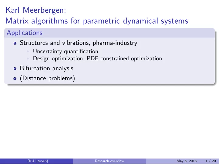
Karl Meerbergen: Matrix algorithms for parametric dynamical systems Applications Structures and vibrations, pharma-industry ◮ Uncertainty quantification ◮ Design optimization, PDE constrained optimization Bifurcation analysis (Distance problems) (KU Leuven) Research overview May 6, 2015 1 / 20

Karl Meerbergen: Matrix algorithms for parametric dynamical systems Applications Structures and vibrations, pharma-industry ◮ Uncertainty quantification ◮ Design optimization, PDE constrained optimization Bifurcation analysis (Distance problems) Linear algebra problems Eigenvalue problems: linear, non-linear Model reduction: linear, non-linear Linear systems: preconditioning Tensors (KU Leuven) Research overview May 6, 2015 1 / 20

Karl Meerbergen: Matrix algorithms for parametric dynamical systems Applications Structures and vibrations, pharma-industry ◮ Uncertainty quantification ◮ Design optimization, PDE constrained optimization Bifurcation analysis (Distance problems) Linear algebra problems Exascale computing Eigenvalue problems: linear, Flanders ExaScience Lab non-linear (Intel) founded in June Model reduction: linear, 2010. non-linear Co-design lab for future Linear systems: preconditioning hardware for HPC Tensors (KU Leuven) Research overview May 6, 2015 1 / 20

Parametric matrices in uncertainty analysis/optimization k = 60 q = 30 − −10 10 Full QMMR −11 10 −12 10 | y | [m 2 /(rad/s) 2 ] −13 10 −14 10 −15 10 −16 10 0 5 10 15 20 25 30 35 40 f [Hz] Large linear systems depending on parameters (frequency, physical parameters) ◮ Preconditioning for indefinite systems (= hard) ◮ Many linear systems to solve − → parametric model reduction Eigenvalue problem depending on (physical) parameters ◮ Eigenvalues play an important role in the dynamics of such problem ◮ Parametric modal truncation: Maryam Saadvandi, Wim Desmet (mechanical engineering) (KU Leuven) Research overview May 6, 2015 2 / 20

Recycling/ Quadratic output SISO linear system ( K − ω 2 M ) x = f x ∗ Sx = y with S symmetric. (Joint with Van Beeumen, Van Nimmen, Lombaert) Method: ◮ Krylov space with f ⇒ V k = [ v 1 , . . . , v k ] ◮ Extract Ritz vectors (M. & Bai) ◮ Use combination of modal superposition (recycle Ritz vectors) with block Krylov for SV k 3 10 2 10 1 10 | y | 0 10 −1 10 −2 10 (KU Leuven) Research overview May 6, 2015 3 / 20 | y | | y | | y |

Dominant poles for nonlinear frequency dependent models SISO Nonlinear system A ( s ) x = fu ( s ) d T x y = For many problems, y can be developed in a modal expansion ∞ R j � y = s − λ j j =1 where λ j is a root of det( A ( s )) = 0. Dominant pole algorithm makes a reduced model based on the dominant terms: k R j � y ≈ s − λ j j =1 Joint work with Maryam Saadvandi and Wim Desmet (Mechanical engineering): compute dominant poles for parametric systems (KU Leuven) Research overview May 6, 2015 4 / 20

Dominant poles for parametric equations � � (1 + 0 . 02 i ) K 0 + ( k 1 + i ω c 1 ) K 1 − ω 2 M � = x f c ∗ x . y = −4 10 γ (1) # iterations time (min) γ (2) γ (3) γ (1) 8 0.45 −5 γ (4) 10 γ (2) 4 0.25 |H(i ω )| γ (3) 7 0.43 −6 10 γ (4) 3 0.19 Total 22 1.32 −7 10 0 5 10 15 20 25 30 i ω (rad/s) (KU Leuven) Research overview May 6, 2015 5 / 20

Model order reduction (MOR) in optimization context Dynamical system: A ( ω, γ ) x = f d T x y = � ω max | y | 2 d ω = (energy) g ω min Objective: minimize g ( γ ) Model reduction using moment matching = Pad´ e approximation via Krylov methods Allows for cheap computation of g and ∇ γ g Penalty and trust region methods based on error estimation of reduced model (Yao Yue) (KU Leuven) Research overview May 6, 2015 6 / 20

Example of the Lamot footbridge OPTEC Application Problem 4 Lamot bridge finite element model ( n = 25 , 962) The goal is to determine the optimal stiffness and damping coefficient of four bridge dampers (=8 parameters). Computation times: ◮ without reduced modeling: 545 for one function evaluation, 70 function evaluations needed. ◮ with reduced model to evaluate g and ∇ g : 879 sec. ◮ trust region method: 200 sec. ◮ penalty method: 189 sec. (KU Leuven) Research overview May 6, 2015 7 / 20

Minimal maximal eigenvalue Parametric eigenvalue problem A ( x ) u = λ B ( x ) u with x ∈ H ⊂ R m λ 1 (x) 1.4 θ 1 (x) 1.2 1 l(x;v 1 ) 0.8 l(x;v 2 ) 0.6 0.4 0.2 0 −0.2 −15 −10 −5 0 5 10 15 20 A and B symmetric and B positive definite for x ∈ H Largest eigenvalue is a quasi convex function Our numerical method (Jeroen De Vlieger): ◮ subspace projection method (= bundle method) ◮ Solve the projected problem by any method for non-smooth problems or a method that approximates the solution by sequence of a 1D problems ◮ Provably convergent (KU Leuven) Research overview May 6, 2015 8 / 20

Minimal maximal eigenvalue (KU Leuven) Research overview May 6, 2015 9 / 20

Parametric eigenvalue problems for stability analysis Find parameter values p so that A ( p ) x = λ Bx has purely imaginary eigenvalues λ . Is translated to ( A ( p ) ⊗ B + B ⊗ A ( p )) z = 0 Exploit the specific Kronecker structure for efficient solvers Appears to be as efficient as solving eigenvalues of A ( p ) for fixed p Much more efficient than continuation Work with Spence, Elman, Voss, Schroeder, Vandebril (KU Leuven) Research overview May 6, 2015 10 / 20

Nonlinear eigenvalue problems Nonlinear eigenvalues problems arise in many applications: A ( λ ) x = 0 Classical iteration schemes converge to one eigenvalue at a time Approximate A ( λ ) ≃ A 0 + λ A 1 + λ 2 A 2 + · · · Apply Arnoldi’s method to the Companion linearization: several eigenvalues converge at the same time With Michiels, Jarlebring, Van Beeumen 10 exact eigenvalues 0 10 Reciprocal Ritz values 5 | λ − λ * | imag 0 −10 10 −5 −20 10 (KU Leuven) Research overview −10 May 6, 2015 11 / 20 0 20 40 60 80 100 −6 −4 −2 0

Nonlinear eigenvalue problems Rational Krylov method: pole can change Approximate A ( λ ) by Newton interpolation in σ 1 , . . . , σ k A ( λ ) ≃ A 0 n 0 ( λ ) + A 1 n 1 ( λ ) + · · · + A k n k ( λ ) j � n j = ( λ − σ i ) i =1 Rational Krylov method with starting vector v corresponds to moment matching: A ( σ 1 ) − 1 v , A ( σ 2 ) − 1 v , . . . , A ( σ k ) − 1 v are contained in the subspace. (KU Leuven) Research overview May 6, 2015 12 / 20

Nonlinear eigenvalue problems Gun problem: � � � � λ − σ 2 λ − σ 2 F ( λ ) x = 0 = K − λ M + i 1 W 1 + i 2 W 2 x Compute eigenvalues near 5 poles. (KU Leuven) Research overview May 6, 2015 13 / 20

Incomplete multifrontal factorization Large sparse linear system Ax = b where A is given in finite element format: � P e A e P T A = e e ∈E ◮ A e is dense (full) matrix ◮ P e selects degrees of freedom associated with the element Multilevel preconditioning using element structure instead of sparse. D k ≡ diag( � , � , � , � ) D k ≡ � � , � , � , � � IMF (Nick Van Nieuwenhoven) (KU Leuven) Research overview May 6, 2015 14 / 20

Incomplete multifrontal factorization Advantages ◮ Use dense matrices: high throughput ◮ More efficient preconditioner than other multilevel techniques 2D Navier-Stokes equation, flow around obstacle, Reynolds number 4000, 16 128 elems (Q1-Q1), 49 440 unknowns, 1 243 530 nnzs. ILUT(0.6) 10 +02 ILU(5) 10 +01 ARMS(0.1) Norm of residual 10 +00 IMF(2) IMF(4) 10 − 01 10 − 02 10 − 03 10 − 04 10 − 05 10 − 06 0 20 40 60 80 100 120 140 160 Execution time (s) (KU Leuven) Research overview May 6, 2015 15 / 20

Sequentially truncated HOSVD A ≈ ( ˆ U 1 , ˆ U 2 , ˆ U 3 ) · ˆ S ˆ U 3 ˆ ˆ ≈ ˆ U 1 S U 2 A Rank ( r 1 , r 2 , r 3 ) orthogonal Tucker approximation to A ˆ  U 1 ∈ R n 1 × r 1  R n 1     ˆ Columns of U 2 ∈ R n 2 × r 2 can be extended to a basis of R n 2  ˆ  U 3 ∈ R n 3 × r 3 R n 3   (KU Leuven) Research overview May 6, 2015 16 / 20

Compression of simulation results I Results for Nick Vannieuwenhoven’s ST-HOSVD. Compression of numerical solution of the heat equation on a square domain computed by explicit Euler. Tensor of size 101 × 101 × 10001 ( x × y × t ). Partially symmetric, 102 . 0 million non-zeros. T-HOSVD and ST-HOSVD truncated to absolute error of 10 − 4 . (KU Leuven) Research overview May 6, 2015 17 / 20

Compression of simulation results II T-HOSVD ST-HOSVD 8 . 512 · 10 − 5 9 . 587 · 10 − 5 Abs. error Rank (22 , 22 , 20) (22 , 21 , 19) T-HOSVD ST-HOSVD Storage (nb. of values) 214144 203140 Factorization time 2h 46m 1m 14.7s 133x speedup! (KU Leuven) Research overview May 6, 2015 18 / 20