Kalman-Filter Peter W uppen Universit at Hamburg Fakult at f - PowerPoint PPT Presentation
MIN-Fakult at Fachbereich Informatik Universit at Hamburg Kalman-Filter Kalman-Filter Peter W uppen Universit at Hamburg Fakult at f ur Mathematik, Informatik und Naturwissenschaften Fachbereich Informatik Technische
MIN-Fakult¨ at Fachbereich Informatik Universit¨ at Hamburg Kalman-Filter Kalman-Filter Peter W¨ uppen Universit¨ at Hamburg Fakult¨ at f¨ ur Mathematik, Informatik und Naturwissenschaften Fachbereich Informatik Technische Aspekte Multimodaler Systeme 16. November 2014 5wueppen 1
MIN-Fakult¨ at Fachbereich Informatik Universit¨ at Hamburg Kalman-Filter Table of Contents 1. Motivation 2. Kalman-Filter History General principle 3. Example application Underlying system dynamics Initialization Results 4. Extended Kalman-Filter 5. Conclusion 5wueppen 2
MIN-Fakult¨ at Fachbereich Informatik Universit¨ at Hamburg Motivation Kalman-Filter Dealing with inaccuracy ◮ Sensor output in dynamic processes often comes with noise ◮ Relying on the exact values often creates a fairly inaccurate description ◮ Tools needed to appropriately deal with noise and extract useful data from sensors 5wueppen 3
MIN-Fakult¨ at Fachbereich Informatik Universit¨ at Hamburg Motivation Kalman-Filter What is the Kalman-Filter? ◮ Tool to control dynamic processes ◮ Creates estimates of a system’s state based on previous estimates and sensor data ◮ Wide range of applications ◮ Tracking objects ◮ Navigation ◮ Economics ◮ Localization (Robotics) 5wueppen 4
MIN-Fakult¨ at Fachbereich Informatik Universit¨ at Hamburg Kalman-Filter - History Kalman-Filter History ◮ Named after Rudolf Emil K´ alm´ an, co-inventor ◮ First described in 1958 ◮ Found one of its first applications in the Apollo program ◮ Still commonly used for all kinds of navigational tasks 5wueppen 5
MIN-Fakult¨ at Fachbereich Informatik Universit¨ at Hamburg Kalman-Filter - General principle Kalman-Filter Requirements For the most effective usage of the Kalman-Filter the following requirements have to be satisfied: ◮ Measurements of the system are available at a constant rate ◮ The error of the measurements follow a gaussian 0-mean distribution ◮ An accurate model of the process is available The basic Kalman Filter is limited to linear dependencies between state variables for transitions and measurement. 5wueppen 6
MIN-Fakult¨ at Fachbereich Informatik Universit¨ at Hamburg Kalman-Filter - General principle Kalman-Filter General principle ◮ Recursive Algorithm ◮ Two phases per observation ◮ Time Update (Predict) ◮ Create a priori estimate of system state based on prior estimation, control input and system dynamics ◮ Create a priori estimate of the error covariance matrix ◮ Measurement Update (Correct) ◮ Compute the Kalman gain, i.e. how strongly the new measurement is factored in for the final estimation ◮ Create a posteriori estimate of system state based on a priori estimation, Kalman gain and measurement ◮ Update the state error convariance matrix, i.e. the confidence in the new estimation 5wueppen 7
MIN-Fakult¨ at Fachbereich Informatik Universit¨ at Hamburg Kalman-Filter - General principle Kalman-Filter From [WB95] 5wueppen 8
MIN-Fakult¨ at Fachbereich Informatik Universit¨ at Hamburg Kalman-Filter - General principle Kalman-Filter Definition x − : A priori estimated state ˆ ˆ : A posteriori estimated state x A : State transition matrix B : Control matrix u : Control input P − : State error covariance matrix Q : Process error covariance matrix K : Kalman gain : Measurement matrix H R : Measurement error covariance matrix : Measurement values z 5wueppen 9
MIN-Fakult¨ at Fachbereich Informatik Universit¨ at Hamburg Example application - Underlying system dynamics Kalman-Filter Example application ◮ We observe the firing of a cannonball at a 45 ◦ angle ◮ Four measurement values: Velocities and positions (x & y) ◮ Measurements are subject to errors (gaussian white noise) ◮ Goal: Precise estimation of the trajectory of the cannonball 5wueppen 10
MIN-Fakult¨ at Fachbereich Informatik Universit¨ at Hamburg Example application - Underlying system dynamics Kalman-Filter Underlying system dynamics We obviously know how the laws of physics will affect the cannonball during its flight: Definition x n = x n − 1 + V x n − 1 ∗ ∆ t V x n = V x n − 1 y n = y n − 1 + V y n − 1 − 1 2 g ∆ t 2 V y n = V y n − 1 − g ∆ t 5wueppen 11
MIN-Fakult¨ at Fachbereich Informatik Universit¨ at Hamburg Example application - Underlying system dynamics Kalman-Filter State transition matrix Based on these assumptions, we can model the transition matrix A, control Matrix B and control input vector u as follows: 1 ∆ t 0 0 0 1 0 0 A = 0 0 1 ∆ t 0 0 0 1 0 0 0 0 0 0 0 0 0 0 B = ; u = − 1 2 ∆ t 2 0 0 0 g 0 0 0 − ∆ t g 5wueppen 12
MIN-Fakult¨ at Fachbereich Informatik Universit¨ at Hamburg Example application - Initialization Kalman-Filter Initilization We initialize the first state estimate with the starting configuration of the system: 0 100 cos ( π 4 ) x 0 = ˆ 500 100 sin ( π 4 ) Note that the initial estimate for y is way off to demonstrate how fast the filter adjusts it. 5wueppen 13
MIN-Fakult¨ at Fachbereich Informatik Universit¨ at Hamburg Example application - Initialization Kalman-Filter Initilization The initial state and process error covariance matrices P and Q are set as: 1 0 0 0 0 0 0 0 0 1 0 0 0 0 0 0 P = ; Q = 0 0 1 0 0 0 0 0 0 0 0 1 0 0 0 0 5wueppen 14
MIN-Fakult¨ at Fachbereich Informatik Universit¨ at Hamburg Example application - Initialization Kalman-Filter Initilization Since our measurement is in actual units, the measurement matrix H is the identity matrix. We assume a certain amount of measurement noise by initializing R as follows: 1 0 0 0 0 . 2 0 0 0 0 1 0 0 0 0 . 2 0 0 H = ; R = 0 0 1 0 0 0 0 . 2 0 0 0 0 1 0 0 0 0 . 2 5wueppen 15
MIN-Fakult¨ at Fachbereich Informatik Universit¨ at Hamburg Example application - Initialization Kalman-Filter Prediction A new state can now be predicted by x n = A ˆ ˆ x n − 1 + Bu and the estimated covariance matrix follows as n = AP n − 1 A T + Q P − 5wueppen 16
MIN-Fakult¨ at Fachbereich Informatik Universit¨ at Hamburg Example application - Initialization Kalman-Filter Correction After calculating the optimal Kalman gain, the final estimates for the state and covariance follow in the second phase: n H T + R ) − 1 n H T ( HP − K n = P − x n = ˆ ˆ x − n + K n ( z n − H ˆ x − n ) P n = (1 − K n H ) P − k 5wueppen 17
MIN-Fakult¨ at Fachbereich Informatik Universit¨ at Hamburg Example application - Results Kalman-Filter Result From [cze] 5wueppen 18
MIN-Fakult¨ at Fachbereich Informatik Universit¨ at Hamburg Extended Kalman-Filter Kalman-Filter Extended Kalman-Filter ◮ Problem with the regular Kalman-Filter: many system or measurement processes are not linear ◮ The extended Kalman-Filter adresses this problem ◮ State transition function instead of matrix ◮ Not an optimal estimator like the linear version, but often reasonable performance ◮ Standard for navigation systems and GPS 5wueppen 19
MIN-Fakult¨ at Fachbereich Informatik Universit¨ at Hamburg Conclusion Kalman-Filter Conclusion ◮ The Kalman-Filter is a a powerful estimator for dynamic discrete-time systems with process and/or measurement noise ◮ Provides optimal estimations in the linear case and often good ones in the non-linear case ◮ Requires a very exact model of the system dynamics to work well 5wueppen 20
MIN-Fakult¨ at Fachbereich Informatik Universit¨ at Hamburg Conclusion Kalman-Filter Thank you for your attention! 5wueppen 21
MIN-Fakult¨ at Fachbereich Informatik Universit¨ at Hamburg Conclusion Kalman-Filter Bibliography [cze] http://http: //greg.czerniak.info/guides/kalman1/ . Accessed: 2015-11-12. [GA93] Mohinder S. Grewal and Angus P. Andrews. Kalman Filtering: Theory and Practice . Prentice-Hall, Inc., Upper Saddle River, NJ, USA, 1993. [WB95] Greg Welch and Gary Bishop. An introduction to the kalman filter. Technical report, Chapel Hill, NC, USA, 1995. 5wueppen 22
Recommend
More recommend
Explore More Topics
Stay informed with curated content and fresh updates.
