JUST THE MATHS SLIDES NUMBER 18.3 STATISTICS 3 (Measures of - PDF document

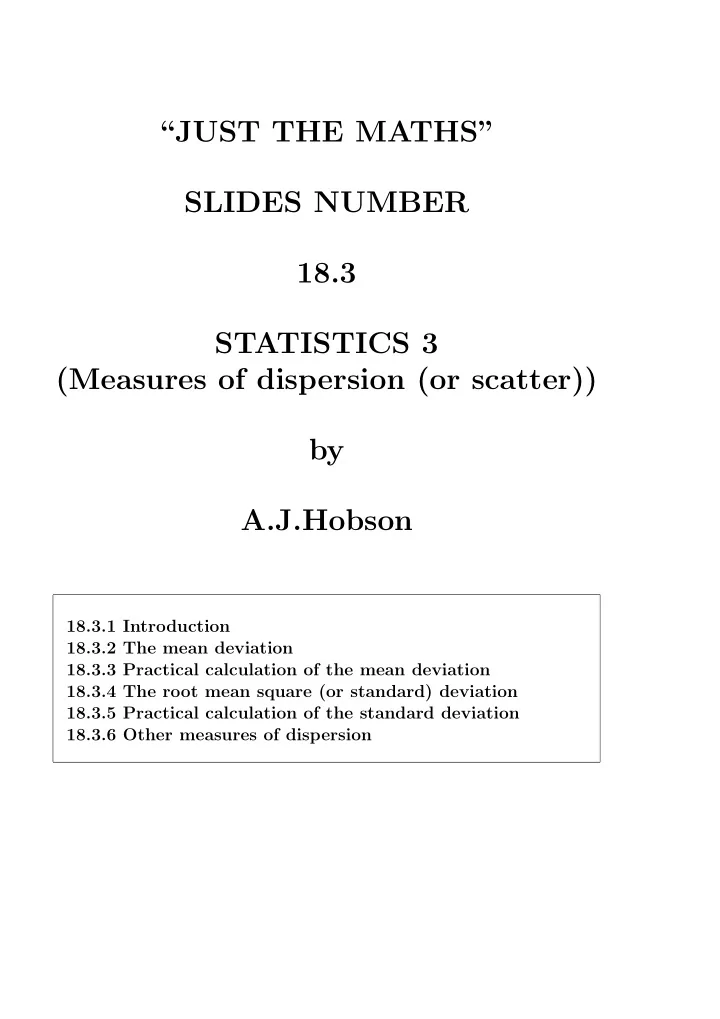
“JUST THE MATHS” SLIDES NUMBER 18.3 STATISTICS 3 (Measures of dispersion (or scatter)) by A.J.Hobson 18.3.1 Introduction 18.3.2 The mean deviation 18.3.3 Practical calculation of the mean deviation 18.3.4 The root mean square (or standard) deviation 18.3.5 Practical calculation of the standard deviation 18.3.6 Other measures of dispersion

UNIT 18.3 - STATISTICS 3 MEASURES OF DISPERSION (OR SCATTER) 18.3.1 INTRODUCTION Averages typify a whole collection of values but give little information about how the values are distributed within the whole collection. For example, 99.9, 100.0, 100.1 is a collection which has an arithmetic mean of 100.0 and so is 99.0,100.0,101.0; but the second collection is more widely dispersed than the first. In this Unit, we examine two types of quantity which typify the distance of all the values in a collection from their arithmetic mean. They are known as “measures of dispersion (or scatter)” and the smaller these quantities are, the more clustered are the values around the arithmetic mean. 1

18.3.2 THE MEAN DEVIATION If the n values x 1 , x 2 , x 3 , ......, x n have an arithmetic mean of x , then x 1 − x , x 2 − x , x 3 − x ,......, x n − x are called the deviations of x 1 , x 2 , x 3 , ......, x n from the arithmetic mean. Note: These deviations add up to zero since n i =1 ( x i − x ) � n n = i =1 x i − i =1 x � � = nx − nx = 0 . DEFINITION The mean deviation ( or, more accurately, the mean ab- solute deviation ) is defined by the formula M . D . = 1 n i =1 | x i − x | . � n 2

18.3.3 PRACTICAL CALCULATION OF THE MEAN DEVIATION In calculating a mean deviation, the following short-cuts usually turn out to be useful, especially for larger collec- tions of values: (a) If a constant, k , is subtracted from each of the val- ues x i (i = 1,2,3... n ), and also we use the “fictitious” arithmetic mean, x − k , in the formula, then the mean deviation is unaffected. Proof: 1 i =1 | x i − x | = 1 n n i =1 | ( x i − k ) − ( x − k ) | . � � n n (b) If we divide each of the values x i (i = 1,2,3,... n ) by a positive constant, l , and also we use the “fictitious” arith- metic mean x l , then the mean deviation will be divided by l . Proof: 1 i =1 | x i − x | = 1 x i l − x n n � � � � � . � � � � � � ln n l � � i =1 � 3

Summary If we code the data using both a subtraction by k and a division by l , the value obtained from the mean deviation formula needs to multiplied by l to give the correct value. 18.3.4 THE ROOT MEAN SQUARE (OR STANDARD) DEVIATION A more common method of measuring dispersion, which ensures that negative deviations from the arithmetic mean do not tend to cancel out positive deviations, is to deter- mine the arithmetic mean of their squares and then take the square root. DEFINITION The “root mean square deviation” ( or “standard deviation” ) is defined by the formula � � 1 � n � i =1 ( x i − x ) 2 . R . M . S . D . = � � � n Notes: (i) The root mean square deviation is usually denoted by the symbol, σ . (ii) The quantity σ 2 is called the “variance” . 18.3.5 PRACTICAL CALCULATION OF 4

THE STANDARD DEVIATION In calculating a standard deviation, the following short- cuts usually turn out to be useful, especially for larger collections of values. (a) If a constant, k , is subtracted from each of the values x i (i = 1,2,3... n ), and also we use the “fictitious” arith- metic mean, x − k , in the formula, then σ is unaffected. Proof: � � 1 � n � i =1 ( x i − x ) 2 � � � n � � 1 � n � i =1 [( x i − k ) − ( x − k )] 2 . = � � � n (b) If we divide each of the values x i (i = 1,2,3,... n ) by a constant, l , and also we use the “fictitious” arithmetic mean x l , then σ will be divided by l . Proof: � � 2 1 � 1 � 1  x i l − x � � n n   i =1 ( x i − x ) 2 = � � � . � � � � �  l n n l i =1 Summary If we code the data using both a subtraction by k and 5

a division by l , the value obtained from the standard deviation formula needs to multiplied by l to give the correct value, σ . (c) For the calculation of the standard deviation, whether by coding or not, a more convenient formula may be ob- tained by expanding out the expression ( x i − x ) 2 as fol- lows: σ 2 = 1  n n n  i =1 x 2 i =1 x 2  . i − 2 x i =1 x i + � � �    n That is, σ 2 = 1 n i − 2 x 2 + x 2 . i =1 x 2 � n This gives the formula � � 1   � n �  − x 2 . i =1 x 2 σ = � �   � i  n Note: In advanced statistical work, the above formulae for stan- dard deviation are used only for descriptive problems in which we know every member of a collection of observa- tions. For inference problems, it may be shown that the stan- dard deviation of a sample is always smaller than that 6

of a total population; and the basic formula used for a sample is � 1 n � � i =1 ( x i − x ) 2 . σ = � � � � n − 1 18.3.6 OTHER MEASURES OF DISPERSION We mention here, briefly, two other measures of disper- sion: (i) The Range This is the difference between the highest and the smallest members of a collection of values. (ii) The Coefficient of Variation This is a quantity which expresses the standard deviation as a percentage of the arithmetic mean. It is given by the formula C . V . = σ x × 100 . 7

EXAMPLE The following grouped frequency distribution table shows the diameter of 98 rivets: f i | x i ′ − x ′ | x i ′ 2 f i x i ′ 2 f i x i ′ Class Cls. Mid Freq Cum ( x i − 6 . 61) / 0 . 02 = x i ′ Intvl. Pt. x i f i Freq. 6 . 60 − 6 . 62 6.61 1 1 0 0 0 0 0.58 6 . 62 − 6 . 64 6.63 4 5 1 4 1 4 2.40 6 . 64 − 6 . 66 6.65 6 11 2 12 4 24 3.72 6 . 66 − 6 . 68 6.67 12 23 3 36 9 108 7.68 6 . 68 − 6 . 70 6.69 5 28 4 20 16 80 3.30 6 . 70 − 6 . 72 6.71 10 38 5 50 25 250 6.80 6 . 72 − 6 . 74 6.73 17 55 6 102 36 612 11.90 6 . 74 − 6 . 76 6.75 10 65 7 70 49 490 7.20 6 . 76 − 6 . 78 6.77 14 79 8 112 64 896 10.36 6 . 78 − 6 . 80 6.79 9 88 9 81 81 729 6.84 6 . 80 − 6 . 82 6.81 7 95 10 70 100 700 5.46 6 . 82 − 6 . 84 6.83 2 97 11 22 121 242 1.60 6 . 84 − 6 . 86 6.85 1 98 12 12 144 144 0.82 Totals 98 591 4279 68.66 Estimate the arithmetic mean, the standard deviation and the mean (absolute) deviation of these diameters. 8

Solution Fictitious arithmetic mean = 591 98 ≃ 6 . 03 Actual arithmetic mean = 6 . 03 × 0 . 02 + 6 . 61 ≃ 6 . 73 � � 4279 � 98 − 6 . 03 2 ≃ 2 . 70 � Fictitious standard deviation = � � Actual standard deviation = 2 . 70 × 0 . 02 ≃ 0 . 054 Fictitious mean deviation = 68 . 66 ≃ 0 . 70 98 Actual mean deviation ≃ 0 . 70 × 0 . 02 ≃ 0 . 014 9