Just Sort It! A Simple and E ff ective Approach to Active Preference - PowerPoint PPT Presentation
Just Sort It! A Simple and E ff ective Approach to Active Preference Learning Lucas Maystre, Matthias Grossglauser School of Computer and Communication Sciences, EPFL ICML August 8 th , 2017 Goal Learning a ranking from noisy pairwise
Just Sort It! A Simple and E ff ective Approach to Active Preference Learning Lucas Maystre, Matthias Grossglauser School of Computer and Communication Sciences, EPFL ICML — August 8 th , 2017
Goal Learning a ranking from noisy pairwise comparisons . some outcomes are inconsistent with the ranking Recover the ranking accurately , but sample sparingly . choose pairs of items adaptively based on previous observations 2
... 3
Main Idea Use a sorting algorithm ! Ground-truth ranking Random ranking Outputs of Quicksort with noise Quicksort Quicksort Quicksort ML estimator ML estimate ranking 4
Why Sorting-based AL ? Prior work : greedy active learning strategies [Houlsby et al. NIPS 2012 , Chen et al. WSDM 2013 , Wang et al. KDD 2014 , ...] r details. Time (in seconds) to select the n +1-st T [s] pair among n items n = 10 2 n = 10 3 n = 10 4 Strategy uncertainty 0 . 05 0 . 5 11 entropy 0 . 3 40 — ε < 10 -5 KL-divergence 0 . 9 71 — orders of magnitude faster Mergesort ε ε ε Quicksort ε ε ε random ε ε ε ... and simpler to implement 5
This Work Theory Practice Accuracy of output of single call to Empirical evaluation of sorting- Quicksort based active learning on real data vs. Quicksort Quicksort Quicksort ML estimator ranking 6
Noise Model Bradley-Terry model [Zermelo 1928 , Bradley & Terry 1952 ] 1 p ( i � j ) = 1 + e − ( θ i − θ j ) θ 1 θ 2 θ 3 R error is likely error is unlikely 7
Sorting Algorithm We analyze Quicksort . 2 5 5 4 7 1 3 6 2 4 1 1 3 5 7 6 6 1 2 4 3 3 5 6 7 1 2 3 4 5 6 7 8
Model Parameters 1 p ( i � j ) = 1 + e − ( θ i − θ j ) Di ff iculty of ranking the items We assume that parameters are depends on | θ 2 - θ 1 |, | θ 3 - θ 2 |, ... drawn from a Poisson point process . Our approach : postulate a i.i.d. θ i +1 − θ i ∼ Exp( λ ) distribution over the parameters s.t. n = 20 E [ | θ i +1 − θ i | ] = λ − 1 controls the average amount of noise 9
Main Result We measure the rank displacement of Theorem : if noise is Bradley-Terry and Quicksort's output σ . i.i.d. θ i +1 − θ i ∼ Exp( λ ) n X with high probability, ∆ ( σ ) = | σ ( i ) − i | i =1 ∆ ( σ ) = O ( λ 2 n ) Rank of item i in Quicksort's output with high probability, True rank of item i max | σ ( i ) − i | = O ( λ log n ) i 10
Sketch of Proof Lemma : Displacement of Quicksort's w.h.p., ∆ ( σ ) = O ( λ 2 n ) output can be bounded by a sum over “individual errors” . ( 1 if outcome is incorrect z ij = 0 otherwise X ∆ ( σ ) ≤ 2 | i − j | comparison pair ( i,j ) ∈ E X E [ ∆ ( σ )] ≤ 2 | i − j | E [ z ij ] pairs sampled by Quicksort i<j that resulted in an error ∞ X k E [ z i,i + k ] = O ( λ 2 n ) ≤ 2 n Does not assume anything about the k =1 noise generating process. decreases exponentially fast in k 11
Experimental Results Sushi dataset GIFGIF dataset × 10 6 1 . 6 2500 uncertainty Mergesort 1 . 4 Quicksort entropy 2000 KL-div random 1 . 2 Mergesort Displacement 1 . 0 Quicksort 1500 random 0 . 8 1000 0 . 6 0 . 4 500 0 . 2 0 0 . 0 0 2000 4000 6000 8000 10000 0 . 1 0 . 2 0 . 3 0 . 4 0 . 5 0 . 6 0 . 7 0 . 8 0 . 9 1 . 0 × 10 6 Number of comparisons c Number of comparisons c Matches the performance of alternatives at a fraction of computational cost . 12
Conclusions • Use sorting algorithms to learn a GIFGIF dataset ranking from noisy comparisons! • works well in practice • computationally inexpensive • Some theoretical results under assumptions on the noise 6170 animated GIF images 2.7+ million pairwise comparisons 13
14
How To Select Comparison Pairs? Batch setting Sequential setting Role of the spectral gap of the Greedy active learning strategies (EIG, comparison graph . uncertainty sampling, ...) [Negahban et al. NIPS 2012 ] [Houlsby et al. NIPS 2012 ] [Hajek et al. NIPS 2014 ] [Chen et al. WSDM 2013 ] [Vojnovic et al. ICML 2016 ] [Ailon et al. NIPS 2011 ] Bandit approaches [Szörényi et al. NIPS 2015 ] [Heckel et al. arXiv 2016 ] Dueling bandits [Yue et al. COLT 2009 ] 15
Empirical Validation max i | σ ( i ) − i | ∆ ( σ ) × 10 4 9 100 8 λ = 2 λ = 2 80 7 λ = 4 λ = 4 6 λ = 6 λ = 6 60 5 λ = 8 λ = 8 4 40 3 2 20 1 0 0 10 1 10 2 10 3 10 4 10 5 0 2000 4000 6000 8000 10000 Number of items n Number of items n 16
Practical AL Strategy In practice : comparison budget is more than that of a single call to Quicksort. ∆ ( ˆ σ ) 900 800 Copeland 700 ML estimate 600 n = 200, λ = 4.0 500 400 300 200 100 0 0 20 40 60 80 100 Number of runs m 17
Recommend
More recommend
Explore More Topics
Stay informed with curated content and fresh updates.
