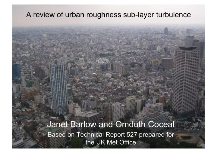

A review of urban roughness sub-layer turbulence Janet Barlow and Omduth Coceal Based on Technical Report 527 prepared for the UK Met Office
H/W = 0.6 Isolated roughness H/W < 0.3 Wake interference 0.3 < H/W < 0.65 Skimming flow H/W > 0.65 H/W = 1.0 Oke, 1988
too complex?! Field studies Physical modelling stability no traffic resolution issues realistic sources idealised layouts and sinks high Re whole domain too simple?! repeatable stationary Numerical modelling 2D: street canyons/bar roughness/cavity flow 3D regular: cubes/cuboids 3D complex: “real” geometry
Papers reviewed on urban RSL flow Field Phys. Num. total mod. mod. 2D 13 6 19 38 3D 3 10 23 36 regular 3D 12 3 1 16 complex total 28 19 43 90 • Papers with significant study of flow within RSL • Mainly flow and momentum exchange rather than scalars
Talk Structure Are common features emerging? • Rough-wall Boundary Layer flow • Canopy flow • Scaling • Urban Morphology • Current modelling approaches • Conclusions and open questions
Rough-wall boundary layer flow
Flow over smooth/rough surfaces (Raupach et al 1991) Boundary layer depth δ Inertial sublayer: friction velocity u* outer layer For rough surface, ADD Inertial sublayer: friction velocity u* Roughness element lengthscales h, L X , L Y , spacing inner layer Viscous lengthscale • Jimenez (2004) flow over rough walls: h/ δ < 0.025 • Castro et al. (2006): urban areas = flow over “very rough walls”? • Review: mean h/ δ = 0.11, range 0.03 to 0.24
Atmospheric Boundary Layer windspeed potential z temperature z i ~1km boundary layer mixed layer ~0.1z i inertial sublayer surface layer ~2-5h Roughness sublayer
RSL depth • Raupach et al 1991: depth 2-5h • Can be 10-15h in unstable conditions (Roth 2000) • Rotach 1995: RSL can “squeeze out” ISL • Cheng and Castro 2002: is there sufficient fetch to grow an ISL? • Cheng et al. 2007: no ISL detected for λ f =0.0625 (aligned cubes)
The BUBBLE project (Basel, Switzerland) Feddersen, 2005, PhD thesis Christen, 2005, PhD thesis Wind tunnel model of Basel Basel-Sperrstra β e tower
• Criterion: height of min. scatter in stress profiles; stress near constant with height above this • Depth = 3.3h ± 0.6h • cf. fullscale: Stress near constant for z > 1.5h, max. height of measurement 2.2h
Canopy flow
Spatial variability within urban canopy Velocity Turbulent kinetic energy Shear stress Dispersive stress Coceal et al. (2007b), z = 0.25h staggered aligned
Spatial mean cf. spatial standard deviation? Significant dispersive stress within canopy
• Velocity moments vary strongly with height in vegetation canopies (“family portrait”, Raupach et al. 1996)
• Christen 2005, “The Basel Family” • Integral lengthscales minimum near urban canopy top • Coceal et al. 2007b: mixing length at minimum near canopy top
Mixing layer hypothesis (Raupach et al 1996) • Inflection point in mean wind profile unstable, leads to growth of coherent structures • Responsible for mixing throughout vegetation canopy depth • Turbulence highly efficient (e.g. R uw > surface layer values)
• Mixing layer analogy yields universal result for vegetation canopies • Turbulence scales on vorticity thickness δ ω • Test for urban canopies?
Coherent structures: field study evidence • Feigenwinter et al. (2005) in Basel • Ensemble averaged coherent structure • Ejection-sweep cycle • Temperature microfront • Oikawa and Meng 1995, Salmond et al. 2004, Christen et al. 2007 • Quadrant analysis and skewness profiles: sweeps dominate within canopy, ejections above
Coherent structures: modelling • Coceal et al. 2007c: “cartoon” • Kanda 2006a, Coceal et al. 2007c, Castro et al. 2006, Inagaki and Kanda 2008 • Consensus not yet reached about coherent structures over urban surfaces – form, generation Structures detected in the field at a single point using wavelet analysis – comparable to EOF analysis of 3D datasets? Most modelling results obtained over uniform sized roughness elements
Scaling velocity and height
Feigenwinter 2005: mean in “constant stress layer” Moriwaki and Kanda 2006d: a) scaled with top measurement b) stress extrapolated to z=h • Cheng and Castro 2002: Better scaling of log law profile using surface stress derived from a) form drag b) average of ISL and RSL stress profile KK and Rotach 2004: peak stress
• Schultz (2007) – left, idealised cube type surface • Kastner-Klein and Rotach (2004) – right, model of Nantes in wind tunnel Peak stress not at z = h, nearer maximum height of buildings Peak stress present in individual profiles – insufficient spatial sampling?
Taller buildings’ contribution to drag • Xie et al. 2008 (based on Cheng and Castro 2002, non-uniform layout): tallest buildings contribute significantly to drag Peak stress parameterisation too sensitive to local tall building influence?
Urban Morphology (or, why did we ever expect buildings to be like trees in the first place…?)
Layout Can we formulate a morphological parameter to quantify element layout? e.g. “gap ratio”? (pic – thanks Anil Padhra) Kanda 2006a: LES, staggered layout higher drag MacDonald 1998: parameterisation includes factor to “correct” drag of individual roughness elements
Wind direction Studies only now emerging showing systematically effect of wind direction changes on flow, drag, dispersion • Kim and Baik 2004 – RANS modelling shows change in mean flow patterns
Urban areas contain other things too… • DAPPLE site (London, UK) • Trees as roughness elements Gromke and Rock 2007: wind tunnel simulation of trees and dispersion Pardyjak 2009: adding canopy to QUIC- URB • Traffic Kastner-Klein et al 2003: parameterisation of TKE due to traffic Pic courtesy of Microsoft Virtual Earth (thanks to Ahmed Balogun)
Current modelling approaches 1) Urban canopy models MacDonald et al. 2000a: Simple Assumes constant mixing length in canopy Bentham and Britter 2003: Simpler!! Assumes no height variation in canopy windspeed Martilli et al. 2002: Can implement in e.g. NWP models What is Cd? Belcher et al. 2003; Coceal and Belcher 2003/4: Allows for adjusting flows What is cd(z)?
Current modelling approaches 2) Empirical parameterisations MacDonald et al. 1998 (z 0 /h, d/h) Simple Based on cubes Rotach 2001: Based on shear stress max, clear feature …assuming there is one! Kastner-Klein and Rotach 2004: Based on shear stress displacement ht Doesn’t include BL depth
Current modelling approaches 3) Models based on mean flow structure Caton et al. 2003: Simple, based on street canyon vortex No unsteadiness represented Dobre et al. 2005: Street canyon vortex, allows for wind direction change Only applicable to “street canyon” type flows Brown; Pardyjak; Addepalli et al. 2007 QUIC-URB: Based on mean flow patterns, apply mass consistency Relies on robust mean flow features, simplistic turbulent exchange
Conclusions: (very) rough surface? • Fetch may not be long enough for an ISL to form. Is h/ δ relevant? • RSL depth observations fall into 2-5H. Definition of depth can be local (single profile) or neighbourhood (spatial average of profiles). Relationship with morphology not clear, e.g. height variability increases RSL depth • Nature of coherent structures not yet established for a range of morphologies – form, production mechanism?
Conclusions: canopy? • Spatial averaging impossible to achieve with fullscale data – substitute averaging over wind directions • Large spatial variability, large bluff elements, large wake size. Need to explore greater range of morphology parameters • Flows are similar in some respects (“The Basel Family Portrait” from BUBBLE). Scaling parameters?? • BUT mixing layer analogy not yet tested fully (behaviour of lengthscales different near canopy top). Model of turbulent production?
Barlow, J.F. and Coceal, O. (2009) A review of urban roughness sub-layer turbulence, Technical Report 527, UK Met Office http://www.metoffice.gov.uk/publications/ NWP papers and reports (registration needed)
Recommend
More recommend