Iterative Methods and Sparse Linear Algebra David Bindel 03 Nov - PowerPoint PPT Presentation
Iterative Methods and Sparse Linear Algebra David Bindel 03 Nov 2015 Logistics I Should be working on shortest paths (on main cores OK for the moment) I Still need to look into Amplifier and MPI issues I You should let me know your final project
Iterative Methods and Sparse Linear Algebra David Bindel 03 Nov 2015
Logistics I Should be working on shortest paths (on main cores OK for the moment) I Still need to look into Amplifier and MPI issues I You should let me know your final project group
Reminder: World of Linear Algebra I Dense methods I Direct representation of matrices with simple data structures (no need for indexing data structure) I Mostly O ( n 3 ) factorization algorithms I Sparse direct methods I Direct representation, keep only the nonzeros I Factorization costs depend on problem structure (1D cheap; 2D reasonable; 3D gets expensive; not easy to give a general rule, and NP hard to order for optimal sparsity) I Robust, but hard to scale to large 3D problems I Iterative methods I Only need y = Ax (maybe y = A T x ) I Produce successively better (?) approximations I Good convergence depends on preconditioning I Best preconditioners are often hard to parallelize
Linear Algebra Software: MATLAB % Dense (LAPACK) [L,U] = lu(A); x = U\(L\b); % Sparse direct (UMFPACK + COLAMD) [L,U,P,Q] = lu(A); x = Q*(U\(L\(P*b))); % Sparse iterative (PCG + incomplete Cholesky) tol = 1e-6; maxit = 500; R = cholinc(A,’0’); x = pcg(A,b,tol,maxit,R’,R);
Linear Algebra Software: the Wider World I Dense: LAPACK, ScaLAPACK, PLAPACK I Sparse direct: UMFPACK, TAUCS, SuperLU, MUMPS, Pardiso, SPOOLES, ... I Sparse iterative: too many! I Sparse mega-libraries I PETSc (Argonne, object-oriented C) I Trilinos (Sandia, C++) I Good references: I Templates for the Solution of Linear Systems (on Netlib) I Survey on “Parallel Linear Algebra Software” (Eijkhout, Langou, Dongarra – look on Netlib) I ACTS collection at NERSC
Software Strategies: Dense Case Assuming you want to use (vs develop) dense LA code: I Learn enough to identify right algorithm (e.g. is it symmetric? definite? banded? etc) I Learn high-level organizational ideas I Make sure you have a good BLAS I Call LAPACK/ScaLAPACK! I For n large: wait a while
Software Strategies: Sparse Direct Case Assuming you want to use (vs develop) sparse LA code I Identify right algorithm (mainly Cholesky vs LU) I Get a good solver (often from list) I You don’t want to roll your own! I Order your unknowns for sparsity I Again, good to use someone else’s software! I For n large, 3D: get lots of memory and wait
Software Strategies: Sparse Iterative Case Assuming you want to use (vs develop) sparse LA software... I Identify a good algorithm (GMRES? CG?) I Pick a good preconditioner I Often helps to know the application I ... and to know how the solvers work! I Play with parameters, preconditioner variants, etc... I Swear until you get acceptable convergence? I Repeat for the next variation on the problem Frameworks (e.g. PETSc or Trilinos) speed experimentation.
Software Strategies: Stacking Solvers (Typical) example from a bone modeling package: I Outer load stepping loop I Newton method corrector for each load step I Preconditioned CG for linear system I Multigrid preconditioner I Sparse direct solver for coarse-grid solve (UMFPACK) I LAPACK/BLAS under that First three are high level — I used a scripting language (Lua).
Iterative Idea x 0 f f x 1 x 2 x ∗ x ∗ x ∗ I f is a contraction if k f ( x ) � f ( y ) k < k x � y k . I f has a unique fixed point x ∗ = f ( x ∗ ) . I For x k + 1 = f ( x k ) , x k ! x ∗ . I If k f ( x ) � f ( y ) k < α k x � y k , α < 1, for all x , y , then k x k � x ∗ k < α k k x � x ∗ k I Looks good if α not too near 1...
Stationary Iterations Write Ax = b as A = M � K ; get fixed point of Mx k + 1 = Kx k + b or x k + 1 = ( M − 1 K ) x k + M − 1 b . I Convergence if ρ ( M − 1 K ) < 1 I Best case for convergence: M = A I Cheapest case: M = I I Realistic: choose something between Jacobi M = diag ( A ) Gauss-Seidel M = tril ( A )
Reminder: Discretized 2D Poisson Problem − 1 j+1 4 j − 1 − 1 j − 1 − 1 i − 1 i i+1 ( Lu ) i , j = h − 2 � � 4 u i , j � u i − 1 , j � u i + 1 , j � u i , j − 1 � u i , j + 1
Jacobi on 2D Poisson Assuming homogeneous Dirichlet boundary conditions for step = 1:nsteps for i = 2:n-1 for j = 2:n-1 u_next(i,j) = ... ( u(i,j+1) + u(i,j-1) + ... u(i-1,j) + u(i+1,j) )/4 - ... h^2*f(i,j)/4; end end u = u_next; end Basically do some averaging at each step.
Parallel version (5 point stencil) Boundary values: white Data on P0: green Ghost cell data: blue
Parallel version (9 point stencil) Boundary values: white Data on P0: green Ghost cell data: blue
Parallel version (5 point stencil) Communicate ghost cells before each step.
Parallel version (9 point stencil) Communicate in two phases (EW, NS) to get corners.
Gauss-Seidel on 2D Poisson for step = 1:nsteps for i = 2:n-1 for j = 2:n-1 u(i,j) = ... ( u(i,j+1) + u(i,j-1) + ... u(i-1,j) + u(i+1,j) )/4 - ... h^2*f(i,j)/4; end end end Bottom values depend on top; how to parallelize?
Red-Black Gauss-Seidel Red depends only on black, and vice-versa. Generalization: multi-color orderings
Red black Gauss-Seidel step for i = 2:n-1 for j = 2:n-1 if mod(i+j,2) == 0 u(i,j) = ... end end end for i = 2:n-1 for j = 2:n-1 if mod(i+j,2) == 1, u(i,j) = ... end end
Parallel red-black Gauss-Seidel sketch At each step I Send black ghost cells I Update red cells I Send red ghost cells I Update black ghost cells
More Sophistication I Successive over-relaxation (SOR): extrapolate Gauss-Seidel direction I Block Jacobi: let M be a block diagonal matrix from A I Other block variants similar I Alternating Direction Implicit (ADI): alternately solve on vertical lines and horizontal lines I Multigrid These are mostly just the opening act for...
Krylov Subspace Methods What if we only know how to multiply by A ? About all you can do is keep multiplying! n o b , Ab , A 2 b , . . . , A k − 1 b K k ( A , b ) = span . Gives surprisingly useful information!
Example: Conjugate Gradients If A is symmetric and positive definite, Ax = b solves a minimization: φ ( x ) = 1 2 x T Ax � x T b r φ ( x ) = Ax � b . Idea: Minimize φ ( x ) over K k ( A , b ) . Basis for the method of conjugate gradients
Example: GMRES Idea: Minimize k Ax � b k 2 over K k ( A , b ) . Yields Generalized Minimum RESidual (GMRES) method.
Convergence of Krylov Subspace Methods I KSPs are not stationary (no constant fixed-point iteration) I Convergence is surprisingly subtle! I CG convergence upper bound via condition number I Large condition number iff form φ ( x ) has long narrow bowl I Usually happens for Poisson and related problems I Preconditioned problem M − 1 Ax = M − 1 b converges faster? I Whence M ? I From a stationary method? I From a simpler/coarser discretization? I From approximate factorization?
PCG Compute r ( 0 ) = b � Ax for i = 1 , 2 , . . . solve Mz ( i − 1 ) = r ( i − 1 ) ρ i − 1 = ( r ( i − 1 ) ) T z ( i − 1 ) if i == 1 Parallel work: p ( 1 ) = z ( 0 ) I Solve with M else I Product with A β i − 1 = ρ i − 1 / ρ i − 2 I Dot products p ( i ) = z ( i − 1 ) + β i − 1 p ( i − 1 ) I Axpys endif q ( i ) = Ap ( i ) Overlap comm/comp. α i = ρ i − 1 / ( p ( i ) ) T q ( i ) x ( i ) = x ( i − 1 ) + α i p ( i ) r ( i ) = r ( i − 1 ) � α i q ( i ) end
PCG bottlenecks Key: fast solve with M , product with A I Some preconditioners parallelize better! (Jacobi vs Gauss-Seidel) I Balance speed with performance. I Speed for set up of M ? I Speed to apply M after setup? I Cheaper to do two multiplies/solves at once... I Can’t exploit in obvious way — lose stability I Variants allow multiple products — Hoemmen’s thesis I Lots of fiddling possible with M ; what about matvec with A ?
Recommend
More recommend
Explore More Topics
Stay informed with curated content and fresh updates.
