Inverse chirp signals from stellar core collapse in massive scalar - PowerPoint PPT Presentation
Inverse chirp signals from stellar core collapse in massive scalar tensor gravity Ulrich Sperhake C Moore, M Agathos, R Rosca, D Gerosa, C Ott DAMTP, University of Cambridge arXiv: 1708.03651 [gr-qc], 1903.09704 [gr-qc] STAG Research Centre
Inverse chirp signals from stellar core collapse in massive scalar tensor gravity Ulrich Sperhake C Moore, M Agathos, R Rosca, D Gerosa, C Ott DAMTP, University of Cambridge arXiv: 1708.03651 [gr-qc], 1903.09704 [gr-qc] STAG Research Centre Gravity Seminar University of Southampton , 12 Dec 2019 This project has received funding from the European Union’s Horizon 2020 research and innovation programme under the Marie Sk ł odowska-Curie grant agreement No 690904, from H2020-ERC-2014-CoG Grant No. ”MaGRaTh" 646597, from NSF XSEDE Grant No. PHY-090003 and from STFC Consolidator Grant No. ST/L000636/1. 1
Overview Introduction and motivation Theoretical framework Massive scalar-tensor gravity Massive self interacting scalar-tensor gravity Observation strategies Conclusions
1. Introduction and motivation
Do we need a theory beyond GR? When asked what he would do if Eddington’s mission failed… But we have reasons to search for “beyond GR” Renormalization: Requires, e.g., higher curvature terms. GR is low-energy limit of more fundamental theory → Dark energy: Why is so small and why Λ ρ dark ∼ ρ mat Dark matter: “Neptune” or “Vulcan” ?
Scalar tensor theory of gravity Scalars appear naturally in extra-dimensional theories Scalars prominent in cosmology ST theory well-posed; fairly well understood mathematically No-hair theorems limit potential of black-hole spacetimes Matter: Neutron stars, core-collapse ⇒ Best example of smoking gun to date: Spontaneous scalarization Damour & Esposito-Farese PRL 1993 Collapse studies in massless case Novak PRD 1998/1999 Novak & Ibanez ApJ 2000, Gerosa+ CQG 2016
Core-collapse scenario to 0th order Massive stars: M ZAMS = 8 . . . 100 M � Core compressed from to ∼ 1 500 km ∼ 15 km ∼ 10 10 g / cm 3 & 10 15 g / cm 3 to Released gravitational energy: O (10 53 ) erg ∼ 10 51 erg in neutrinos, in outgoing shock, explosion ∼ 99 % Explosion mechanism: still uncertainties… Failed explosions lead to BH formation “Collapsar”: possible engine for long-soft GRBs All of this handled for us by Woosley & Heger Phys.Rept. 2007 Initial pre-collapse profile →
2. Theoretical framework
Theoretical framework Einstein frame: conformal metric g µ ν = F ( ϕ ) g µ ν ¯ Action 1 Z dx 4 √− ¯ g [ ¯ S = R − 2¯ g µ ν ∂ µ ϕ ∂ ν ϕ − 4 V ( ϕ )] + S m [ ψ m , ¯ g µ ν /F ( ϕ )] 16 π Energy momentum tensor: T αβ = ρ hu α u β + Pg αβ s 2 = ¯ g µ ν dx µ dx ν = − F α 2 dt 2 + FX 2 dr 2 + r 2 d Ω 2 Spherical symmetry: d ¯ 1 u α = 1 − v 2 [ α − 1 , vX − 1 , 0 , 0] √ Equations (gravity): ∂ r α = . . . , ∂ r X = . . . ∂ t ∂ t ϕ = . . . Equations (matter): HRSC ( ρ , h, v ) ↔ ( D, S r , τ ) ⇒ GR1D code O’Connor & Ott CQG 2009
Theoretical framework Coupling function Einstein frame: conformal metric F ( ϕ ) g µ ν = F ( ϕ ) g µ ν ¯ Action Potential 1 Z dx 4 √− ¯ g [ ¯ S = R − 2¯ g µ ν ∂ µ ϕ ∂ ν ϕ − 4 V ( ϕ )] + S m [ ψ m , ¯ V ( ϕ ) g µ ν /F ( ϕ )] 16 π Equation of state Energy momentum tensor: T αβ = ρ hu α u β + Pg αβ h P s 2 = ¯ g µ ν dx µ dx ν = − F α 2 dt 2 + FX 2 dr 2 + r 2 d Ω 2 Spherical symmetry: d ¯ 1 u α = 1 − v 2 [ α − 1 , vX − 1 , 0 , 0] √ Equations (gravity): ∂ r α = . . . , ∂ r X = . . . ∂ t ∂ t ϕ = . . . Equations (matter): HRSC ( ρ , h, v ) ↔ ( D, S r , τ ) ⇒ GR1D code O’Connor & Ott CQG 2009
<latexit sha1_base64="LwDNo6hbfsKeU0prb4sSYnKlX0Q=">ACHnicbVBNS8NAEN34bf2qevSyWAXxUJKi6EUQvHhUsCo0tUy2k3ZxNxt2N2I+SVe/CtePCgieNJ/47b24NeDgcd7M8zMi1LBjfX9D29sfGJyanpmtjI3v7C4VF1eOTcq0wybTAmlLyMwKHiCTcutwMtUI8hI4EV0fTwL25QG6SM5un2JbQS3jMGVgndaq7YRyp2Ij7HKTCsiNzQXSUEnsQWf7Iw1sCKUGWVXjbI+xHocqPsVGt+3R+C/iXBiNTICed6lvYVSyTmFgmwJhW4Ke2XYC2nAksK2FmMAV2DT1sOZqARNMuhu+VdNMpXRor7SqxdKh+nyhAGpPLyHVKsH3z2xuI/3mtzMb7YInaWYxYV+L4kxQq+gK9rlGpkVuSPANHe3UtYHl4h1iVZcCMHvl/+S80Y98OvB6U7tcH8UxwxZI+tkiwRkjxySY3JCmoSRO/JAnsizd+89ei/e61frmDeaWSU/4L1/Agvsov4=</latexit> <latexit sha1_base64="LwDNo6hbfsKeU0prb4sSYnKlX0Q=">ACHnicbVBNS8NAEN34bf2qevSyWAXxUJKi6EUQvHhUsCo0tUy2k3ZxNxt2N2I+SVe/CtePCgieNJ/47b24NeDgcd7M8zMi1LBjfX9D29sfGJyanpmtjI3v7C4VF1eOTcq0wybTAmlLyMwKHiCTcutwMtUI8hI4EV0fTwL25QG6SM5un2JbQS3jMGVgndaq7YRyp2Ij7HKTCsiNzQXSUEnsQWf7Iw1sCKUGWVXjbI+xHocqPsVGt+3R+C/iXBiNTICed6lvYVSyTmFgmwJhW4Ke2XYC2nAksK2FmMAV2DT1sOZqARNMuhu+VdNMpXRor7SqxdKh+nyhAGpPLyHVKsH3z2xuI/3mtzMb7YInaWYxYV+L4kxQq+gK9rlGpkVuSPANHe3UtYHl4h1iVZcCMHvl/+S80Y98OvB6U7tcH8UxwxZI+tkiwRkjxySY3JCmoSRO/JAnsizd+89ei/e61frmDeaWSU/4L1/Agvsov4=</latexit> <latexit sha1_base64="LwDNo6hbfsKeU0prb4sSYnKlX0Q=">ACHnicbVBNS8NAEN34bf2qevSyWAXxUJKi6EUQvHhUsCo0tUy2k3ZxNxt2N2I+SVe/CtePCgieNJ/47b24NeDgcd7M8zMi1LBjfX9D29sfGJyanpmtjI3v7C4VF1eOTcq0wybTAmlLyMwKHiCTcutwMtUI8hI4EV0fTwL25QG6SM5un2JbQS3jMGVgndaq7YRyp2Ij7HKTCsiNzQXSUEnsQWf7Iw1sCKUGWVXjbI+xHocqPsVGt+3R+C/iXBiNTICed6lvYVSyTmFgmwJhW4Ke2XYC2nAksK2FmMAV2DT1sOZqARNMuhu+VdNMpXRor7SqxdKh+nyhAGpPLyHVKsH3z2xuI/3mtzMb7YInaWYxYV+L4kxQq+gK9rlGpkVuSPANHe3UtYHl4h1iVZcCMHvl/+S80Y98OvB6U7tcH8UxwxZI+tkiwRkjxySY3JCmoSRO/JAnsizd+89ei/e61frmDeaWSU/4L1/Agvsov4=</latexit> <latexit sha1_base64="LwDNo6hbfsKeU0prb4sSYnKlX0Q=">ACHnicbVBNS8NAEN34bf2qevSyWAXxUJKi6EUQvHhUsCo0tUy2k3ZxNxt2N2I+SVe/CtePCgieNJ/47b24NeDgcd7M8zMi1LBjfX9D29sfGJyanpmtjI3v7C4VF1eOTcq0wybTAmlLyMwKHiCTcutwMtUI8hI4EV0fTwL25QG6SM5un2JbQS3jMGVgndaq7YRyp2Ij7HKTCsiNzQXSUEnsQWf7Iw1sCKUGWVXjbI+xHocqPsVGt+3R+C/iXBiNTICed6lvYVSyTmFgmwJhW4Ke2XYC2nAksK2FmMAV2DT1sOZqARNMuhu+VdNMpXRor7SqxdKh+nyhAGpPLyHVKsH3z2xuI/3mtzMb7YInaWYxYV+L4kxQq+gK9rlGpkVuSPANHe3UtYHl4h1iVZcCMHvl/+S80Y98OvB6U7tcH8UxwxZI+tkiwRkjxySY3JCmoSRO/JAnsizd+89ei/e61frmDeaWSU/4L1/Agvsov4=</latexit> The coupling function and potential Coupling function: F ( ϕ ) = e − 2 α 0 ϕ − β 0 ϕ 2 determine all modifications at 1st PN order α 0 , β 0 Potential for a massive non-interacting scalar field V ( ϕ ) = 1 2 µ 2 ϕ 2 ω ∗ = µc 2 Mass introduces characteristic frequency µ ~ µ = 10 − 14 eV Here typically: ω ∗ = 15 . 2 s − 1 ⇔
Equation of state Pressure: “cold” + “thermal” contribution: P = P c + P th ( K 1 ρ Γ 1 if ρ ≤ ρ nuc Hybrid EOS for cold part: P c = K 2 ρ Γ 2 if ρ > ρ nuc K 1 Γ 1 − 1 ⇢ Γ 1 − 1 if ⇢ ≤ ⇢ nuc Internal energy from 1st law: ✏ c = Γ 2 − 1 ⇢ Γ 2 − 1 + E 3 K 2 if ⇢ > ⇢ nuc Thermal pressure: P th = ( Γ th − 1) ⇢ ( ✏ − ✏ th ) Parameters: Γ 1 = 1 . 3 , Γ 2 = 2 . 5 , Γ th = 1 . 35 K 1 = 4 . 9345 × 10 14 [cgs] , ρ nuc = 2 × 10 14 g cm − 3 from continuity at K 2 , E 3 ρ = ρ nuc
The coupling function and potential Coupling function, potential: V ( ϕ ) = 1 F ( ϕ ) = e − 2 α 0 ϕ − β 0 ϕ 2 2 µ 2 ϕ 2 10 − 2 α 0 10 − 3 PSRJ0348+0432 PSR J1738+0333 Cassini Runs 10 − 4 − 6 − 4 − 2 0 2 4 6 β 0 µ . 10 − 19 eV Only for !! Here: µ [eV] ∈ [10 − 15 , 10 − 12 ] Ramazanoglu & Pretorius PRD 2016 Free parameters: µ, α 0 , β 0 , Γ 1 , Γ 2 , Γ th
Convergence test µ = 10 − 14 eV , α 0 = 10 − 4 , For β 0 = − 20 Γ 1 = 1 . 3 , Γ 2 = 2 . 5 , Γ th = 1 . 35 Using points N 1 = 5000 , N 2 = 10000 , N 3 = 20000 Discretization error: ∼ 5 %
3. Massive ST gravity
Waveforms ``close to’’ the source µ = 10 − 14 eV , α 0 = 10 − 2 , For β 0 = − 20 Γ 1 = 1 . 3 , Γ 2 = 2 . 5 , Γ th = 1 . 35 0 r ex ϕ [cm] 5 -1 × 10 Fiducial -4 α 0 = 10 0 α 0 = 1 -14 eV 5 µ = 3x10 -2 × 10 5 -1 × 10 Γ 2 = 3 α 0 = 1, β 0 = -10 5 -2 × 10 0.1 0.2 0.3 0.4 0.5 5 -3 × 10 0 1 2 3 t [s] massless case; fairly insensitive to parameters; dispersion! r ϕ �
Waveforms ``far from’’ the source LIGO will observe the above scalar profiles after they propagate to large distances In the massless case this is almost trivial ϕ ( t ; r ) = 1 r ϕ ( t − r ; r extract ) In the massive case things are more complicated: signals propagate with dispersion
Waveforms ``far from’’ the source Far from the source, scalar dynamics are governed by the flat-space Klein-Gordon wave equation ∂ 2 t ϕ � r 2 ϕ + ω 2 ∗ ϕ = 0 Easier to work with the radially rescaled field σ ≡ r ϕ As the signal propagates outwards: The scalar field - Low frequencies are suppressed - High frequency power spectrum is unaffected mass has a natural - Signal spreads out in time frequency ω ∗ = c 2 µ/ ~ - High frequencies arrive earlier than low frequencies - Signal becomes increasingly oscillatory
Recommend
More recommend
Explore More Topics
Stay informed with curated content and fresh updates.
