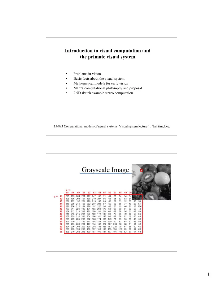
Introduction to visual computation and the primate visual system - PDF document

Introduction to visual computation and the primate visual system • Problems in vision • Basic facts about the visual system • Mathematical models for early vision • Marr’s computational philosophy and proposal • 2.5D sketch example stereo computation 15-883 Computational models of neural systems. Visual system lecture 1. Tai Sing Lee. 15-883 Computational models of neural systems. Visual system lecture 1. Tai Sing Lee. 1

What make vision difficult? 1. Projection of 3D scene into 2D array of numbers - recovering the lost dimension 2. Variability of object manifestations -- invariance 3. Multiple causes for generating images -- disambiguation 4. Occlusion and clutters - figure-ground, attention. What does it mean to understand something What does it mean to understand something computationally? computationally? 1. Computational theory 1. Computational theory 2. Algorithms Algorithms 2. 3. Implementations. 3. Implementations. Marr (1981) Vision. Marr (1981) Vision. David Marr (1945-1980) David Marr (1945-1980) 2

Computational theory Computational theory • • What is the goal of the computation? What is the goal of the computation? • Why is it appropriate? • Why is it appropriate? • • What is the logic of the strategy by which it can What is the logic of the strategy by which it can be carried out? be carried out? 1. 1. Computational constraints Computational constraints 2. 2. Prior knowledge Prior knowledge Representation and algorithms Representation and algorithms • • How can the computational theory be implemented? How can the computational theory be implemented? • What is the representation for the input and output? • What is the representation for the input and output? • • What is the algorithm for the transformation? What is the algorithm for the transformation? 3

Representation and algorithms Representation and algorithms • • How can the computational theory be implemented? How can the computational theory be implemented? • What is the representation for the input and output? • What is the representation for the input and output? • • What is the algorithm for the transformation? What is the algorithm for the transformation? Processes and representations Processes and representations Hardware implementation Hardware implementation • • How can the representation and algorithm be How can the representation and algorithm be realized physically? realized physically? 4

What is known about the visual system at the time? What is known about the visual system at the time? Cajal’s microscopic study of the retina 5

On-off center surround receptive fields of intact retina, cells responded primarily to contrast and to moving stimuli rather than diffused light. Steven Kuffler (1953) John Dowling John Dowling 6

Laplacian of Gaussian operator • DOG (difference of Gaussians) of ratio 1:1.6 best approximates a Laplacian of Gaussian filter ( Marr and Hildreth,1980) Laplacian of Gaussian 2 r � r 2 1 �� 4 (1 � r 2 � � 2 G ( r ) = � 1 2 G ( r ) e 2 = � 2 � 2 2 � 2 ) e � 2 2 �� where r is the radial distance from the origin. where r is the radial distance from the origin. 7

Difference of Gaussian smoothed images *g= *g= *g= *g= - - - - DOG DOG DOG DOG L 0 L 1 Retinal receptive fields and resolution 8

Organization of visual pathways from retina to cortex • Optic Nerve - digital signal • Optic Chiasma • Optic tracts • Lateral geniculate nucleus • Optic radiation • Primary visual cortex (Striate cortex, V1, area 17) • Extrastriate cortex 9

Thalamus LGN anatomy 6 layers sandwiched together: Layers 1 and 2: magnocellular (M) layers, large cells, fast processing and conducting, motion, gross features, monochromatic, transient response. 1 mm 1 mm Layer 3,4,5,6: parvocellular (P) layers, small cell bodies, thin fibre, high-resolution, fine details, sustained responses, color coded. Between layers: unmyelinated neural dendrites and axons, also contains interlaminar or koniocellular (K) layer. Functionally distinct third channels. 10

Functional difference between magnocellular and parvocellular LGN neurons Parvo Magno Color sensitivity High (cones) Low (cones+rods) Contrast sensitivity Low High Spatial resolution High Low Temporal resolution Slow Fast Receptive field size Small Large LGN monocular retinotopic maps from both eyes Input from the right hemi-retina of each eye Input from the right hemi-retina of each eye project orderly to different layers of the right project orderly to different layers of the right LGN to create 6 complete representations of LGN to create 6 complete representations of the left visual hemi-field the left visual hemi-field 11

What are the differences between retinal and LGN neurons? 1. Broad attributes resemble retinal ganglian cells 2. Contrast gain control strengthened. 3. RF with a center and a larger surround. 4. Biphasic temporal kernel in both center and surround. 5. LGN receives feedback, but not retina. Hubel Hubel and and Wiesel Wiesel 12

Ocular dominance columns and hypercolumns Cells tuned to a variety of visual Cells tuned to a variety of visual cues: color, orientation, disparity, cues: color, orientation, disparity, motion direction. motion direction. The actual topological map revealed The actual topological map revealed by optical imaging. by optical imaging. 13

Gabor filters are spatial frequency analyzers Daugman (1985) and others proposed simple cells can be modeled by Gabor filters. Jones and Palmer (1988) confirmed Gabor fit. 14

V1 neurons modeled as Gabor wavelets, wavelets can efficiently encode images Lee (1996) Image representation using 2D Gabor wavelets. PAMI. 18(10): 959-971. Gabor wavelet like structures can be learned as sparse efficient codes wavelet like structures can be learned as sparse efficient codes Gabor from natural image patches -- Olshausen Olshausen and Field (1996), and Field (1996), from natural image patches -- 15

Visual areas in the visual system Visual areas in the visual system Cortical areas flat map 16

Ventral and dorsal streams 17

Object detector neurons in IT Combination Coding and Invariance 18

Marr’s proposal on visual processing Digitized Image Filtering, Edge detection, Chunking Primal Sketch Depth, surfaces, occlusion, figure-ground 2 1/2 D Sketch 3D structural model and parts 3D Model Comparison with memory prototypes Object Recognition /Scene Description Marr’s proposal on visual processing Digitized Image Filtering, Edge detection, Chunking Primal Sketch V1,V2 V1,V2 Depth, surfaces, occlusion, figure-ground 2 1/2 D Sketch V2,V4 V2,V4 3D structural model and parts IT IT 3D Model Comparison with memory prototypes Object Recognition /Scene Description 19

Julesz random dot stereogram Stereo Correspondence is Hard 20

Computing 2.5D sketch -- e.g. stereopsis Computational constraints 1. Compatibility : Black dots can match only black dots. 2. Uniqueness : Almost always, a black dot from one image can match no more than one black dot from the other image. 3. Continuity : The disparity of the matches varies smoothly almost everywhere over the image. Marr and Poggio (Marr 1976). • Left and right eyes • Continuous lines = line of sights • Intersection = possible disparity values • Dotted diagonal lines = lines of constant disparity (planar surface). • How to implement the rules? 21

Iterative (Relaxation) Algorithm t + 1 = � { � t � t 0 C x , y ; d C x ', y ', d ' C x ', y ', d ' + C x , y , d } � � x ', y ', d ' � S ( x , y , d ) x ', y ', d ' � O ( x , y , d ) t where C x , y , d denotes the state of the cell corresponding to the position ( x , y ) , disparity d and time t . It is binary. S ( x , y , d ) is the local excitatory neighborhood, and O ( x , y , d ) is the inhibitory neighborhood. � is the inhibitory constant, and � is the threshold function. C 0 is all the possible matches, including false targets, within the prescribed disparity range, added at each iteration to speed up convergence, can simply use to initialize. See also See also Samonds Samonds, , Potetz Potetz and Lee (2007) NIPS for neural evidence of and Lee (2007) NIPS for neural evidence of the the computational constraints at work during stereo computation. computational constraints at work during stereo computation. 22

Computing 2.5D sketch -- e.g. shape from shading Potetz (2007) (2007) Potetz 3D model Blanz and Vetter (1999) and Vetter (1999) Blanz 23