Introduction to NMR relaxation Jozef Kowalewski Stockholm - PDF document
pNMR Mariapfarr 2014 Introduction to NMR relaxation Jozef Kowalewski Stockholm University Outline What is NMR? Phenomenological Bloch equations Introductory example: spin-lattice relaxation Elements of statistics and theory
pNMR Mariapfarr 2014 Introduction to NMR relaxation Jozef Kowalewski Stockholm University Outline • What is NMR? • Phenomenological Bloch equations • Introductory example: spin-lattice relaxation • Elements of statistics and theory of random processes • Time-dependent perturbation theory • A simple model and its predictions • Dipole-dipole relaxation 1
What is NMR? • Features: Splitting controlled by the experimenter ( B 0 field) Many species possible to study ( I ≠ 0, γ I ), most common is 1 H Very small energy splitting & population difference with the available magnets Atkins et al . ” Quanta, Matter and Change” 1 H NMR of ethanol • What NMR measures in solution: Line positions (chemical shifts) Splittings ( J - couplings) Integrals Relaxation • Relaxation means return to equilibrium after a perturbation 2
Simple NMR: magnetization vector • The equilibrium state of an ensemble of N (non-interacting) spins can be described by a magnetization vector, oriented along B 0 and with the length: 2 2 N I I ( 1) B M I 0 0 3 k T B • The magnetization vector is a classical quantity and can be described by classical physics • Effect of radiofrequency pulses Figures from: Kowalewski & Mäler, ” Nuclear Spin Relaxation in Liquids ”, Taylor & Francis, 2006 Simple relaxation: Bloch equations • Phenomenological • Free induction decay description of the (FID) on resonance magnetization vector decays exponentially after a pulse (in rotating with T 2 , transverse frame): relaxation time dM M x M x y off dt T 2 dM M y y M x off dt T 2 dM M M z 0 z dt T 1 M x , y M 0 exp( t / T 2 ) 3
Spin-lattice relaxation • Consider a sequence of two RF-pulses: (180º-t-90º- FID), called inversion-recovery experiment: M z ( t ) M 0 (1 2exp( t / T 1 )) Meaning of T 1 and T 2 • Longitudinal relaxation ( T 1 ): energy exchange with other degrees of freedom (the lattice) • Transverse relaxation ( T 2 ): loss of phase coherence, gives decay of FID and the line-broadening: 4
Simple theory – spin-lattice relaxation 1. • Consider a system of I =1/2 spins • Energy splitting proportional to B 0 , ω 0 =Larmor frequency • Populations: n α , n β • At equilibrium, Boltzmann distributed: n α eq , n β eq • A non-equilibrium situation can be created by changing the magnetic field or by RF- pulses Simple theory – spin-lattice relaxation 2. • Assume simple kinetics for changing the populations of the two states: dn eq eq n n W n n W dt eq eq W n n n n I dn eq eq W n n n n I dt 5
Simple theory – spin-lattice relaxation 3. • Instead of discussing changes in populations, we introduce the sum ( N ) and difference ( n ) in populations dN 0 dt dn eq 2 W n n I dt Simple theory – spin-lattice relaxation 4. The simple result shows that the dN 0 change in the difference in dt population (return to equilibrium dn eq 2 W n n or relaxation) occurs through an I dt exponential process. If we assume that the difference in population is proportional to the longitudinal component of the magnetization vector, M z ( t ), we can identify from the Bloch equations: 1/T 1 =2W I 6
Transition probabilities • The relaxation rate is proportional to the transition probability • Transitions giving rise to NMR relaxation are non- radiative, they do not arise through emission or absorption of radiation from radiofrequency field • They occur as a result of weak magnetic interactions within the sample, if those oscillate in time with frequency components at the Larmor frequency • Weak interaction → slow relaxation Where do the transitions come from? • Weak magnetic interactions often anisotropic • Time-dependence through molecular motions • The reorientation of molecules (or molecule-fixed axes) can be pictured as a random walk on a sherical surface • The combination of the motion and anisotropic interactions leads to: • Hamiltonians varying randomly with time: stochastic interaction 7
Stochastic variables 1. • The orientation of a molecule-fixed axis can be described in terms of stochastic variables, characterized by probability density p x y dxdy ( ; ) orientation P x ( X x dx y ; Y y dy ) • Means: the probability that X and Y take on values in the indicated ranges Stochastic variables 2. • If p ( x ; y )= p ( x ) p ( y ) we say that the two variables are statistically independent • We can also write: p ( x ; y )= p ( x ) p ( x | y ), the latter meaning the probability that Y takes on the value y provided that X takes on value x conditional probability m X xp x dx ( ) • Average value (mean): 1 • The second moment around the mean (variance): 2 2 2 2 ( X m ) X m 2 1 1 m XY Product of two variables: 11 If the two variables are statistically independent: m XY X Y 11 8
Stochastic variables 3. • The mixed second moment: ( X m ) ( Y m ) XY m m 11 10 01 10 01 • Correlation coefficient: 11 X Y • Vanishes if X and Y statistically independent Stochastic functions of time The time-dependence of anisotropic interactions can be described in terms of stochastic functions of time (stochastic processes) due to the random motions Average value: Y t yp y t dy , The properties of a stochastic function are in general dependent on t . What is the correlation between Y ( t ) at two time- points, t 1 and t 2 ? 9
What is the correlation between Y ( t ) at two time-points, t 1 and t 2 ? “t 1 -t 2 small” “t 1 -t 2 large” •Correlation vanishes for large time separations •The same is true for an ensemble average over many spins Stationary stochastic process If t 1 and t 2 are close (defined by the time-scale of the random oscillation of Y ( t )) a correlation is probable Useful formulation with the conditional probability density for Y ( t ) acquiring the value y 2 at t 2 provided that it takes on y 1 at t 1 : p ( y , t ; y , t ) p ( y , t ) p ( y , t | y , t ) 1 1 2 2 1 1 1 1 2 2 If the probability p ( y 1 , t 1 ) density does NOT vary with time, the process is called stationary . In such a case: p ( y , t | y , t ) p ( y , 0 | y , t t ) p y | y , 1 1 2 2 1 2 2 1 1 2 10
Time-correlation functions The average value of a product of a stationary process, Y ( t ) at two different times can be defined. Because this quantity is only dependent on the time difference, t = t 2 - t 1 , we can define: Y ( t ) Y ( t ) G ( t t ) G ( ) 1 2 2 1 Time-correlation function (TCF) Autocorrelation function: The same function correlated with itself at different time points. Acts as a correlation coefficient between the same stochastic variable at different points in time. Cross-correlation function: Different functions at different points in time are correlated Properties of time-correlation functions The autocorrelation function of Y at t =0 becomes the variance of Y : 2 2 G ( 0 ) Y ( t ) Y * ( t ) | Y ( t ) | The average of Y ( t ) can often be assumed to be zero. Reasonable to assume that correlation vanishes for long . lim G 0 The following TCF works (and can be derived within a simple model): G G 0 exp / c The correlation time, τ c , can be interpreted as a measure of persistence of the correlation of the values Y ( t ) at different points in time. 11
Illustration of correlations on different time-scales “short correlation time” “long correlation time” Correlation function Correlation function Size and temperature dependence of correlation time One can use hydrodynamic arguments to derive the Stokes-Einstein-Debye relationship for a sphere: 3 4 a V a = radius 3 c k T k T = viscosity B B This relation is valid for a rank-2 spherical harmonics •Correlation time increases with molecular size •Correlation time increases with viscosity •Correlation time decreases with temperature The temperature dependence is often modeled by an Arrhenius-type expression: exp E / k T c 0 a B 12
Spectral density functions Spectral density functions are Fourier transforms of the time-correlation functions. J 2 G exp i d 0 From the exponentially decaying time-correlation function we get a Lorentzian spectral density 2 J G (0)1 c 2 2 c Spectral density functions The spectral density function as a function of frequency calculated with different correlation times. Corrrelation time 0.5 ns 2 ns 5 ns -10 -5 0 5 10 (rad/s)/10 9 13
Recommend
More recommend
Explore More Topics
Stay informed with curated content and fresh updates.
