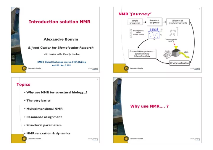
Introduction solution NMR Alexandre Bonvin Bijvoet Center for - PowerPoint PPT Presentation

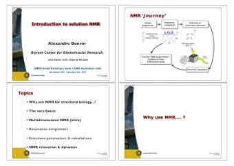
2 NMR ‘ journey ’ Introduction solution NMR Alexandre Bonvin Bijvoet Center for Biomolecular Research with thanks to Dr. Klaartje Houben EMBO Global Exchange course, IHEP, Beijing April 28 - May 5, 2011 3 Topics • Why use NMR for structural biology...? • The very basics Why use NMR.... ? • Multidimensional NMR • Resonance assignment • Structural parameters • NMR relaxation & dynamics

5 6 NMR & Structural biology NMR & Structural biology CBD apo-CAP CAP-cAMP 2 b c Dynamic activation of an allosteric regulatory protein Tzeng S-R & Kalodimos CG Nature (2009) High-resolution multidimensional NMR spectroscopy of proteins in human cells Inomata K. et al Nature (2009) ...allows to study the dynamics of ...structural studies in membrane and biomolecular systems... whole cells possible! 7 8 Pros & cons of solution NMR in The Sample structural biology • isotope labeling • Pros... – unlabeled (peptides) – no need for crystal: – 15 N labelled (small proteins < 10 kDa) • no crystal packing artefacts, solution more native-like – potential to study dynamics: – 15 N & 13 C labelled (larger proteins, up to 30-40 kDa) • picosecond to seconds time scales, conformational averaging, – 15 N, 13 C & 2 H labelled (large proteins > 40 kDa) chemical reactions, folding... – easy study of protein-protein, protein-DNA, protein- • protein production ( E.coli ) ligand interactions – quite a lot & very pure & stable • Cons... • 500 uL of 0.5 mM solution -> ~ 5 mg per sample – NMR structure determination is a bit slow.... – 13 C labelling is costly, ~k ! per sample – Need isotope labeling ( 13 C, 15 N) – preferably low salt, low pH, no additives. – solution NMR works best for MW < 50 kDa

10 The very basics of NMR 11 12 Nuclear spin Nuclear spin precession (rad . T -1 . s -1 ) E = µ B 0

13 14 Larmor frequency Boltzman distribution Larmor frequency 1 H (I = 1/2) 1 H (I = 1/2) ! H = " H B 0 = 2 #$ H m = - ! m = - ! m = ! m = ! 15 16 Net magnetization Chemical shielding Local magnetic field is influenced by electronic environment

17 18 Chemical shielding Chemical shift # B ( ) Chemical shielding • Chemical shift: $ = % ! 0 1 " – δσ iso [Hz] = ν obs - ν 0 2 – δσ iso [ppm] = ( ν obs - ν 0 )/( ν 0. 10 -6 ) 14 Tesla: ! H = 600 MHz → 1 ppm = 600 Hz ( 1 H) • ppm: parts per million • ppm value is not field dependent 21 Tesla: ! H = 900 MHz → 1 ppm = 900 Hz ( 1 H) 19 20 Pulse FID: analogue vs digital Observe with the Lamor frequency → “rotating frame” Free Induction Decay ( FID )

21 22 Fourier Transform Relaxation • NMR Relaxation Signal Signal – Restoring Boltzmann equilibrium FT 0 0 0 50 75 100 125 200 0 5 10 15 20 25 30 35 40 25 150 175 freq. (s -1 ) time (ms) • T2-relaxation – disappearance of transverse (x,y) magnetization – 1/T2 ~ signal line-width • T1-relaxation FT – build-up of longitudinal (z) magnetization – determines how long you should wait for the next experiment 23 24 NMR spectral quality Scalar coupling / J-coupling • Sensitivity – Signal to noise ratio (S/N) • Sample concentration • Field strength H 3 C - CH 2 - Br • .. • Resolution 3 J HH – Peak separation • Line-width (T2) • Field strength • ..

26 Why multidimensional NMR • multidimensional NMR experiments – resolve overlapping signals • enables assignment of all signals Multidimensional NMR – encode structural and/or dynamical information • enables structure determination • enables study of dynamics 27 28 2D NMR 3D NMR

29 30 nD experiment Encoding information direct dimension 1D • mixing/magnetization transfer single FID of N points t 1 FID indirect dimensions ???? 2D E = E = N FIDs of N points t 2 t 1 mixing FID proton A proton B 3D NxN FIDs of N points spin-spin interactions t 3 t 1 t 2 mixing mixing FID 31 32 Magnetization transfer homonuclear NMR NOESY magnetic dipole • magnetic dipole interaction (NOE) t m t 1 t 2 interaction crosspeak intensity ~1/r 6 – Nuclear Overhauser Effect up to 5 Å FID – through space – distance dependent (1/r6) – NOESY -> distance restraints COSY t 1 J-coupling interaction t 2 transfer over one J-coupling, i.e. • J-coupling interaction max. 3-4 bonds FID – through 3-4 bonds max. – chemical connectivities – assignment TOCSY – also conformation dependent J-coupling interaction t 1 t 2 transfer over several J-couplings, i.e. multiple steps over max. 3-4 mlev FID bonds

33 34 homonuclear NMR 2D COSY & TOCSY ~Å E = E = NOESY proton B t 2 proton A t 1 t m FID 2D COSY 2D TOCSY A A ( ω A ) A A ( ω A ) (F1,F2) = ω A, ω A H β H β B ( ω B ) (F1,F2) = ω A, ω B B ω A ω B H α H α Diagonal F1 H N H N ω A Cross-peak F2 35 36 heteronuclear NMR J coupling constants E = E = 1 J CbCg = 35 Hz 1 J CbHb = 130 Hz 1 H 15 N 1 J CaCb = 35 Hz 1 J CaC’ = 1 J NC’ = 1 J CaN = – measure frequencies of different nuclei; e.g. 1 H, 15 N, 13 C 55 Hz -15 Hz -11 Hz – no diagonal peaks 1 J CaHa = 140 Hz – mixing not possible using NOE, only via J 1 J HN = -92 Hz 2 J CaN = 7 Hz 2 J NC’ < 1 Hz

37 38 J coupling constants heteronuclear NMR HSQC (heteronuclear single quantum coherence) t 2 1 H FID J-mix J-mix block block t 1 15 N DEC 1 J NH 1 J NH 15 N ( ω 15 N ) 1 H 1 H ( ω 1 H ) (F 1 ,F 2 ) = ω 15 N , ω 1 H 1 J HN = -92 Hz 39 40 1 H- 15 N HSQC: ‘ protein fingerprint ’ 1 H- 15 N HSQC: ‘ protein fingerprint ’ note that spectrum is decoupled: no NH J- coupling

41 42 J coupling constants Triple resonance NMR HNCA t 3 1 H FID J-mix J-mix block block t 2 15 N DEC 1 J CaN = -11 Hz J-mix J-mix block block t 1 13 C 2 J CaN = 7 Hz 1 J NH 1 J NCa(i) 1 J NCa(i) 1 J NH 15 N 1 H 13 C ( ω 13 C ) 15 N ( ω 15 N ) 1 H ( ω 1 H ) 2 J NCa(i-1) 2 J NCa(i-1) (F 1 ,F 2 ,F 3 )= ( ω 13 Ca(i) , ω 15 N(i) , ω 1 H(i) ) & ( ω 13 Ca(i-1) , ω 15 N(i) , ω 1 H(i) ) 1 J HN = -92 Hz Resonance assignment Structural parameters

Structural study by NMR Sources of structural information • OBSERVABLES • Sample preparation ( months ) – chemical shifts ( 1 H, 15 N, 13 C, 31 P) • Acquisition of NMR spectra (~ 1 Secondary structure – J-couplings, e.g. J(H N ,H α ) month ) • Chemical shift assignments – long-range NOEs Tertiary structure – residual dipolar couplings – Backbone ( days ) – Side-chains ( days ) – H / D exchange • Analysis of NOESY spectra ( weeks ) RESTRAINTS – effects of pH / T • Structure calculations ( days ) ! dihedral angles a few – effects of interacting partners ! distances between months or – relaxation rates atoms more... • Functional studies with NMR ! orientation between – ..... bond vectors – Interaction with partner 47 48 RESTRAINTS: dihedral angles RESTRAINTS: dihedral angles anti-parallel β -strand α -helix ω ~ 180º C C ψ N C C N C C φ ψ ω φ O O φ ψ φ φ

49 50 Ramachandran plot OBSERVABLE: chemical shift +180 • 13 C α and 13 C β chemical shifts β -strand – sensitive to dihedral angles – report on secondary structure elements ψ β -strand α -helix φ -130 -60 α -helix ψ 125 -45 -180 -180 φ +180 51 52 OBSERVABLE: homonuclear J- RESTRAINT: distances couplings Karplus J = A.cos 2 ( φ ) + B.cos ( φ ) + C φ φ ! ! measured 3 J(H N H α ) reports on φ

53 54 OBSERVABLE: NOE OBSERVABLE: NOE r = • 1 H- 1 H NOEs (2D NOESY, 3D NOESY-HSQC) • 1 H- 1 H NOEs r = – signal intensity proportional to 1/r 6 – signal intensity proportional to 1/r 6 – reports on distance between protons – reports on distance between protons • distance restraints • distance restraints Sequential Intra-residue ( used for identifying A B C • • • • D Z spin-systems ) H y Medium range H x Sequential & medium range NOEs - SECONDARY STRUCTURE Cross-peak between H x and H y 55 56 NOEs in secondary structure OBSERVABLE: NOE elements • 1 H- 1 H NOES – signal intensity proportional to 1/r 6 – reports on distance between protons • distance restraints Longe range Sequential Intra-residue ( used for identifying • • • • A B C D Z spin-systems ) Medium range Long range NOEs - TERTIARY STRUCTURE

57 58 Long-range NOEs RESTRAINT: Orientation • Tertiary information – distances < 5 Å – Important structural information anti-parallel 59 60 OBSERVABLE: Residual dipolar OBSERVABLE: Residual dipolar couplings couplings 3cos 2 % ( t ) " 1 3cos 2 % ( t ) " 1 D ij = " # i # j ! µ 0 D ij = " # i # j ! µ 0 Dipolar coupling Dipolar coupling 4 $ 2 r 3 4 $ 2 r 3 2 2 B 0 B 0 Ω No protein alignment No protein alignment Protein alignment ISOTROPIC SYSTEM ISOTROPIC SYSTEM ANISOTROPIC SYSTEM D = 0 D = 0 D ≠ 0