Introduction to microarrays Thierry Sengstag, PhD Bioinformatics - - PowerPoint PPT Presentation

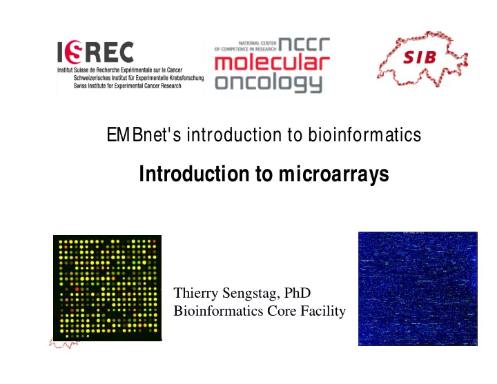
EMBnet's introduction to bioinformatics

Introduction to microarrays

Thierry Sengstag, PhD Bioinformatics Core Facility

Part I

Technology of microarrays

Biology Fundamentals - Genes

Biology Fundamentals - Expression

Transcriptome: Genes Proteome: Proteins

Microarrays

Genomics Fundamentals - Complexity

Difficulties: §Contaminations §Alternative Splicing §Alternative PolyAdenylation mRNA purification

RNA abundance in mammalian cells

rRNA tRNA

mRNA

80%

1%

1-50 50-500 500+ Molecules/cell 3 x 106 molecules/cell 3 x 105 molecules/cell 1-2 x104 different genes

DNA microarray is a technology that allows scientists to simultaneously detect thousands of genes in a small sample and to analyze the expression of those genes. Microarrays are ordered sets of DNA molecules of known sequence attached on a surface at a known position (spot). In a microarray experiment one hybridizes mRNA molecules of an extract of a sample to the spots of the microarray. Main families of microarrays:

• Spotted arrays, PCR products spotted on chip, ~500 nt
• Oligo-arrays, e.g. Agilent, oligos ~60 nt length, in-situ
• Affymetrix, short sequence oligos, 25 nt, in-situ

What are DNA Microarrays ?

1- Samples 2- Extracting mRNA 3- Labeling 4- Hybridizing 5- Scanning 6- Visualizing

Various technological choices:

• 104 to 106 features on a single array
• Single- vs two-color approach
• Hybridization protocols

Questions addressed:

• What are the differences (in gene expression) between cell lines ?
• What is the difference between knock-out and wild-type mice?
• What is the difference between a tumor and a healthy tissue ?
• Are there different tumor types ?

Key concept: Compare gene expression in two (or more) cell/tissue types ? Gene expression assessed by measuring the number of RNA transcripts in a tissue sample. (Primary goal of this course.)

What are DNA Microarrays ?

Phase 1: Preparation of the microarray environment

• Which sequences do we want to interrogate on the arrays ?
• Other technically important questions (choice of scanner,

chemistry, etc…)

• Presently (2006): commercial platforms are standard for

"usual" organisms; "exotic" organisms still require custom-made arrays Phase 2: Use of the microarray

• "Experimental design" (with a statistician)
• Preparation of RNA samples
• Hybridization, scanning, signal extraction
• Statistical analysis

Two major phases of a microarray experiment

Phase 1: Which sequences should we spot ?

Depends on the organism:

• Human, Mouse, Rat, … have large databases of sequences that

can be used to design probes by bioinformatics means

• "Exotic" organisms require cloning of 100s to 1000s mRNA

transcripts, then spotting of DNA after PCR amplification (sequencing of interesting genes can be done after microarray experiment)

Depends on platform:

• Oligo arrays can probe any region of a mRNA transcript
• Affymetrix require the sequence to be in the 3'-UTR region

Biological question (e.g. Differentially expressed genes, Sample class prediction, etc.)

Testing

Biological verification and interpretation Microarray experiment

Significance

Experimental design Image analysis/ Quality assessment Normalization

Clustering Discrimination

(failed) Pre-processing steps Data Analysis

Scientific Process

Phase 2:

Spotted array preparation

“Average” mouse mRNA cDNA isolation Test sequence (probe) production

~100 - ~2000 bp RT-PCR (conversion mRNA-cDNA, amplification)

Array Production: Spotting

Spotting in action…

1. Some rounds of pin cleaning 2. Pickup PCR products from plate 3. Spot one feature on each subarray Spotting arrays

Oligo array preparation

Sequence databases Millions of experiences worldwide Probe (sequence) design

• known genes
• putative genes
• alternative splicing
• GC contents

Gene-specific sequences

~60 bp sequences

In-situ synthesis

Spotted and oligo array usage

Hybridization washing

Relative mRNA levels

Scanning cy5 labeled cDNA cy3 labeled cDNA

Mix

Affymetrix chip preparation

Sequence databases Millions of experiments worldwide Probe (sequence) design

• known genes
• putative genes
• alternative splicing
• GC contents

Bioinformatics thinking yields gene-specific sequences (3’-end)

25 nt sequences

In-situ synthesis

~100s of nt “consensus” sequences

Affymetrix chip usage

Hybridization washing Relative mRNA levels Scanning Scanning

Affymetrix system

(11 to 16)

Usually the most 3 prime area, often UTR

25mer 25mer 25mer

AAAA. .

25mer

Probe preparation & hybridization

• Extract mRNA or total RNA
• RT, add 5’ anchor
• PCR with labelled nucleotide (Cy3, Cy5, DIG, …)
• Overlay probe on the chip, put in the hybridization

chamber, wash

Scanner basics

• Based on fluorescence

– 1 or 2 lasers: cy3 cy5 (seldom more)

• Most scanners are confocal

– Target a very limited volume

• f space

(signal only from focal plane) – Need to “scan” the surface

• 16-bits ADC converters

– Range of values: 0-65535 – Log2 range: 0 – 16

• Scan various supports

– Glass Slide (e.g. Agilent, PerkinElmer) – Affymetrix

Confocal scanner

Dye Photons Electrons Signal Laser PMT A/D Converter excitation amplification Filtering Time-space averaging

Images from Scanner

• Resolution

– standard 10 µm [currently, best ~ 5µm] – 100µm spot on chip = 10 pixels in diameter

• Image format

– Typically: TIFF (tagged image file format) 16 bit (65,536 levels of gray) – also other formats – 1cm x 1cm image at 16 bit = 2Mb

• Separate image for each fluorescent sample

– channel 1, channel 2, etc.

Images in analysis software

• The two 16-bit images (Cy3, Cy5) are viewed as 8-bit

images

• Display fluorescence intensities for both wavelengths

using a 24-bit RGB overlay image

• RGB image :

– Blue values (B) are set to 0 – Red values (R) are used for Cy5 intensities – Green values (G) are used for Cy3 intensities

• Qualitative representation of results

Images : examples

Cy3 Cy5 repressed Control > Treated green induced Control < Treated red unchanged Control = Treated yellow

Gene expression Signal strength Spot color

Image analysis (scanner variability)

ScanArray 4000 Agilent G2565AA

Image processing

• Align channels
• Identify spot pixels
• Identify background pixels
• Compute representative value, e.g.

– Mean foreground value – Median background value

2-color Arrays Image Processing

GenePix

2-color Arrays Image Processing

A difficult case… J J J J

Quantification of Expression

For each spot on the slide, calculate Red intensity = Rfg - Rbg (fg = foreground, bg = background) and Green intensity = Gfg - Gbg and combine them in the log (base 2) ratio Log2(Red/Green) Often, fg = mean and bg = median of relevant pixel intensities

M and A values

• M-value is the log2 of the ratio of expression values

– Properties:

• If the gene is expressed with the same intensity in the red

and green conditions: M=0

• If the gene is more expressed in the red condition: M>0
• if the gene is more expressed in the green condition: M<0
• A-value is the average of the log2 of expression

M = log2( Red / Green )

= log2( Red ) – log2( Green )

A = 1/2 ( log2( Red ) + log2( Green ) )

= log2( sqrt( Red * Green ) )

Why we take logs

Linear scale Log scale

Better representation of genes with "medium" expression: Biologically, a unit change in log2 represents a 2-fold change.

MvA plots

• Relationship between Intensity and MvA plots

log2(Green) log2(Red) 16 16 M A 16 45o Rotation

Red saturation Red saturation Green saturation Green saturation

+1

• 1

(+ stretching by a factor 2 along M axis)

Hybridization of extra material with known concentrations (spikes)

A real-life MvA plot

End of Part I

Part II

Extraction of gene signal from microarrays

Biological question (e.g. Differentially expressed genes, Sample class prediction, etc.)

Testing

Biological verification and interpretation Microarray experiment

Significance

Experimental design Image analysis/ Quality assessment Normalization

Clustering Discrimination

(failed) Pre-processing steps Data Analysis

Scientific Process

Steps in Images Processing

• Addressing (or Gridding)

– Assigning coordinates to each spot

• Segmentation

– Classification of pixels as either foreground (signal)

• r background
• Information Extraction

– Foreground fluorescence intensity pairs (R,G) – Background intensities – Quality measures

Addressing

This is the process of assigning coordinates to each of the spots. Automating this part of the procedure permits high throughput analysis.

4 by 4 grids 19 by 21 spots per grid

Addressing

Problems in automatic addressing

• Misregistration of the red and green channels
• Rotation of the array in the image

Rotat i

• n

Rotat i

• n

Problems in automatic addressing

• Skew in the array

• Parameters to address spot positions

– Separation between rows and columns of grids – Individual translation of grids – Separation between rows and columns of spots within each grid – Small individual translation of spots – Overall position of the array in the image

Addressing

• Basic structure of images known

(determined by the arrayer)

Steps in Images Processing

• Addressing (or Gridding)

– Assigning coordinates to each spot

• Segmentation

– Classification of pixels as either foreground (signal)

• r background
• Information Extraction

– Foreground fluorescence intensity pairs (R,G) – Background intensities – Quality measures

Segmentation Methods

• Fixed circles
• Adaptive circles
• Adaptive shape

– Edge detection – Seeded Region Growing (R. Adams and L. Bishof (1994): Regions grow outwards from seed points preferentially according to the difference between a pixel’s value and the running mean of values in an adjoining region

• Histogram methods

Fixed circle segmentation

• Fits a circle with a constant diameter to all spots in

the image

• Easy to implement
• The spots should be of the same shape and size

Adaptive circle segmentation

• The circle diameter is

estimated separately for each spot

Dapple finds spots by detecting edges of spots (second derivative)

• Problematic if spot

exhibits oval shapes

Limitation of circular segmentation

—Small spot —Not circular

Result of Seed Region Growing

Adaptive shape segmentation

• Specification of starting points or seeds

– Bonus: already know geometry of array

• Regions grow outwards from the seed points

preferentially according to the difference between a pixel’s value and the running mean

• f values in an adjoining region

Histogram segmentation

• Choose target mask larger than any spot
• Fg and bg intensities determined from the

histogram of pixel values for pixels within the masked area

• Example : QuantArray

– Background : mean between 5th and 20th percentile – Foreground : mean between 80th and 95th percentile

• May not work well when a large

target mask is set to compensate for variation in spot size ! "

Steps in Images Processing

• Addressing (or Gridding)

– Assigning coordinates to each spot

• Segmentation

– Classification of pixels as either foreground (signal)

• r background
• Information Extraction

– Foreground fluorescence intensity pairs (R,G) – Background intensities – Quality measures

Information Extraction

• Spot Intensities

§ mean of pixel intensities § median of pixel intensities § Pixel variation (e.g. IQR)

• Background values

§ None § Local § Constant (global)

• Quality Information

Take the average

Spot ‘foreground’ intensity

• The total amount of hybridization for a spot is

proportional to the total fluorescence generated by the spot

• Spot intensity = sum of pixel intensities within

the spot mask

• Since later calculations are based on ratios

between Cy5 and Cy3, we compute the average* pixel value over the spot mask

*alternative : ratios of medians may be better than means if bright specks present

Background intensity

• The measured fluorescence intensity includes

a contribution of non-specific hybridization and other chemicals on the glass

• Fluorescence from regions not occupied by

DNA should be different from regions

• ccupied by DNA

→ one solution is to use local negative controls (spotted DNA that should not hybridize)

BG: None

• Do not consider the background

– Can be better than some forms of local background determination with good quality arrays

        + − + + − + =

bg G bg fg G fg bg R bg fg R fg

G G R R M

, , , , 2

log σ σ σ σ

        + + + + ≈ ) ( ) ( log

, , , , 2 bg G fg G fg bg R fg R fg

G R σ σ σ σ

With a loose mathematical notation:

        + + =

fg G fg fg R fg

G R M

, , 2

log σ σ worse than

BG: Local

• Focus on small regions surrounding the spot mask
• Median of pixel values in this region
• Most software implements such an approach

#$ %$

• By ignoring pixels immediately surrounding the

spots, bg estimate is less sensitive to the performance of the segmentation procedure

Background can matter

Without BG correction With BG correction

Summary

• Image analysis is a crucial preprocessing step

– Association of a "geographic" location (and corresponding annotation) with signal intensities – Several non-trivial technical choices (scanner, image analysis software, etc…) can affect the quality of the signal

• Bg correction is sometimes not desirable

(low bg arrays)

Biological question (e.g. Differentially expressed genes, Sample class prediction, etc.)

Testing

Biological verification and interpretation Microarray experiment

Significance

Experimental design Image analysis/ Quality assessment Normalization

Clustering Discrimination

(failed) Pre-processing steps Data Analysis

Scientific Process

Quality assessment overview Visual inspection of images Evaluation of MvA plots Compare statistical summaries for the chips

$& '%(( & %% ((

Co-registration and overlay offers a quick visualization, revealing information on color balance, uniformity of hybridization, spot uniformity, background, and artifacts such as dust or scratches

Red/Green overlay images

Spatial plots: background from two slides

Practical Problems 1

Comet Tails

§ Likely cause: insufficiently rapid immersion

• f the slides in

the succinic anhydride blocking solution

Practical Problems 2

% ) %

Practical Problems 3

High Background

• 2 likely causes:

– Insufficient blocking – Precipitation of the labeled probe

Weak Signals

Practical Problems 4

• § *!&

+

Practical Problems 5

Artifacts in microarrays

• We are interested in finding true biologically

meaningful differences between sample types

• Due to other sources of systematic variation,

there are also usually artifactual differences

• Sources of artifacts include:

– print tips - differences in subarrays – plate effects – differences in rows within subarray – batch effects – hybridization artifacts

Sample boxplot

• ,-

,. /'!0

*.1&2+%2# 34

Boxplots of log2R/G

(Example data associated to limmaGUI package.)

Biological question (e.g. Differentially expressed genes, Sample class prediction, etc.)

Testing

Biological verification and interpretation Microarray experiment

Estimation

Experimental design Image analysis/ Quality assessment Normalization

Clustering Discrimination

(failed) Pre-processing steps Data Analysis

Scientific Process

Pin group (sub-array) effects

Boxplots, highlighting pin group effects

Clear example of spatial bias

• *

Preprocessing: Normalization

• Why?

To correct for systematic differences between samples

• n the same slide, or between slides, which do not

represent true biological variation between samples

• How do we know it is necessary?

By examining self-self hybridizations, where no true differential expression is occurring. There are dye biases which vary with spot intensity, location on the array, plate origin, pins, scanning parameters, etc.

What is self-self hybridization?

• In dual channel (2-color) microarrays, such as

cDNA arrays, two samples are each labeled with a different fluorescent dye

• In most studies, the samples are from different

sources (e.g. cancer vs. normal)

• However, it is also possible to co-hybridize two

samples from the same source (but differently labeled)

Dual channel co-hybridizations

(self-self) Control sample Treated sample Control sample Control sample

False color overlay Boxplots within pin-groups Scatter (MA-)plots

Self-self hybridizations

Normalization: global

• Normalization based on a global adjustment

log2 R/G → log2 R/G - c = log2 R/(kG)

• Common choices for k or c = log2k are c =

median or mean of log ratios for a particular gene set (e.g. all genes, or control, or ‘housekeeping’ genes)

• Another possibility is total intensity

normalization, where k = ∑Ri/ ∑Gi

Effect of global normalization

Normalization: intensity-dependent

• Here, run a line through the middle of the MA

plot, shifting the M value of the pair (A,M) by c=c(A), i.e. log2 R/G → log2 R/G - c (A) = log2 R/(k(A)G)

• One estimate of c(A) is made using the LOWESS

(or loess) function of Cleveland (1979): LOcally WEighted Scatterplot Smoothing

Effect of lowess normalization

Comparison between arrays

• Different arrays often do not show identical signal

distribution of M values

– Various technical reasons (e.g. labeling efficiency, amount of labelled RNA, scanner settings, etc…)

• Need to normalize the signal

between chips

– Multiple possibilities, one

• ften used: "scale normalization"

Boxplots of log ratios from 3 replicate self-self hybs Left panel: before normalization Middle panel: after within print-tip group normalization Right panel: after a further between-slide scale normalization

Scale normalization: between slides

Idea: make the median spread of M values identical by multiplying them by a chip-specific constant

Assume: All slides have the same spread in M

• True log ratio is mij where i represents different

slides and j represents different spots

• Observed is Mij, where Mij = ai mij
• Robust estimate of ai is

MADi = medianj { |mij - median(mij) | }

• Could instead make same assumption for print tip

groups (rather than slides)

Taking scale into account

NCI 60 experiments

Same normalization on another data set

Normalization: Summary

• Reduces systematic (not random) effects
• Makes it possible to compare several arrays
• Use logratios (MVA plots)
• Lowess normalization (dye bias)
• Pin-group location normalization
• Pin-group scale normalization
• Between slide scale normalization
• Control Spots
• Normalization introduces more variability
• Outliers (bad spots) handled with replication

cDNA gene expression data

Data on p genes for n samples:

$ 56 78

$ 78 9 56*:5 7 ;$6

sample1 sample2 sample3 sample4 sample5 …

1 0.46 0.30 0.80 1.51 0.90 ... 2

• 0.10

0.49 0.24 0.06 0.46 ... 3 0.15 0.74 0.04 0.10 0.20 ... 4

• 0.45
• 1.03
• 0.79
• 0.56
• 0.32

... 5

• 0.06

1.06 1.35 1.09

• 1.09

...

Software for Microarray Analysis

• Very large number of commercial and free

softwares (GeneSpring, PathwayAssist,…)

• There are several R packages for microarray

analysis available as part of the open source BioConductor project http://www.bioconductor.org/

• BioC software often created by the author of

the methodology

Biological question (e.g. Differentially expressed genes, Sample class prediction, etc.)

Testing

Biological verification and interpretation Microarray experiment

Significance

Experimental design Image analysis/ Quality assessment Normalization

Clustering Discrimination

(failed) Pre-processing steps Data Analysis

Scientific Process

cDNA gene expression data

Data on p genes for n samples:

$ 56 78

$ 78 9 56*:5 7 ;$6

sample1 sample2 sample3 sample4 sample5 …

1 0.46 0.30 0.80 1.51 0.90 ... 2

• 0.10

0.49 0.24 0.06 0.46 ... 3 0.15 0.74 0.04 0.10 0.20 ... 4

• 0.45
• 1.03
• 0.79
• 0.56
• 0.32

... 5

• 0.06

1.06 1.35 1.09

• 1.09

...

Replicated experiments

• Have n replicates
• For each gene, have n values of M = log2 fold

change, one from each array

• Summarize M1, ..., Mn for each gene by

– M = average (M1, ..., Mn) – s = SD(M1, ..., Mn)

• Rank genes in order of strength of evidence in favor
• f DE
• How might we do this?

Which genes are DE?

• Difficult to judge significance

– massive multiple testing problem – genes dependent – don’t know null distribution of M

• Strategy

– aim to rank genes – assume most genes are not DE (depending on type of experiment and array) – find genes separated from the majority

Ranking criteria

• Genes i = 1, ..., p
• Mi = average log2 fold change for gene i

– Problem : genes with large variability likely to be selected, even if not DE

• Fix that by taking variability into account:

use ti = Mi/ (si/√n)

– Problem : genes with extremely small variances make very large t – When the number of replicates is small, the smallest si are likely to be underestimates

Summary

• Image analysis is important to extract information

from the array

– Background may or may not be taken into account

• Normalization procedures are always needed

– To remove systematic (technical) effects – To allow comparisons between chips

• Identification of differentially expressed genes is

difficult

– No absolute estimation of significance is possible – Ranking of genes by significance is possible

End of part II

Part III

Higher-level analysis

Finding biological information

Once the matrix of gene-expression vs samples is available, statistical tools can be used to:

• Find similarity (or difference) of expression pattern in

differentially expressed genes

• Find differentially expressed functional groups of genes

(pathway analysis, gene ontology)

• Find classes in the set of samples

(unsupervised analysis)

• Use differentially expressed genes as a mean to classify

samples in known categories (supervised analysis)

• Find genes significantly related to survival in a pool of patients

Unsupervised analysis: Cluster analysis

• data matrix (n,p)
• distance matrix (n,n),

similarity matrix (n,n)

• cluster formation:

– mutually exclusive clusters – hierarchical clusters

• comparison of

clusters, means and variances

Dendrogram

Hierarchical Clustering (real case)

Sorlie et al. Proc Natl Acad Sci U S A 2001 Sep 11;98(19):10869-74

Unsupervised analysis: PCA

• Principal Components Analysis

(PCA)

• Columns (resp. rows) of

expression matrix viewed as points in multidimensional space

• Find “dominant” directions in

space and hope these directions can be associated with known parameters

• Genes (resp. samples) with largest

projection on those vectors explain the parameter

X1 X2 PC1 PC2 X1 X2

Supervised analysis example: KNN

• Based on a measure of distance between observations (e.g.

Euclidean distance or one minus correlation)

• k-nearest neighbor rule (Fix and Hodges (1951)) classifies an
• bservation X as follows:

– find the k observations in the learning set closest to X – predict the class of X by majority vote, i.e., choose the class that is most common among those k observations.

• The number of neighbors k can be chosen by cross-validation

?

Gene 1 Gene 2 k-Nearest Neighbor (knn)

Data Matrix

Gene Sample

High-level analysis (summary)

• Needed to extract biological information after

low-level processing conducted

• Can be used to:

– Discover new interactions between genes (unsupervised analysis) – Validate biological hypotheses (supervised analysis)

• Contact your local statistician for more on this

topic !

End of Part III