Introduction to Information Retrieval - PowerPoint PPT Presentation
Introduction to Information Retrieval http://informationretrieval.org IIR 1: Boolean Retrieval Hinrich Sch utze Center for Information and Language Processing, University of Munich 2014-04-09 1 / 60 Boolean retrieval The Boolean model is
Normalization Need to “normalize” words in indexed text as well as query terms into the same form. Example: We want to match U.S.A. and USA We most commonly implicitly define equivalence classes of terms. Alternatively: do asymmetric expansion window → window, windows windows → Windows, windows Windows (no expansion) More powerful, but less efficient Why don’t you want to put window , Window , windows , and Windows in the same equivalence class? 17 / 62
Normalization: Other languages Normalization and language detection interact. PETER WILL NICHT MIT. → MIT = mit He got his PhD from MIT. → MIT � = mit 18 / 62
Tokenization: Recall construction of inverted index Input: Friends, Romans, countrymen. So let it be with Caesar . . . Output: friend roman countryman so . . . Each token is a candidate for a postings entry. What are valid tokens to emit? 19 / 62
Exercises In June, the dog likes to chase the cat in the barn. – How many word tokens? How many word types? Why tokenization is difficult – even in English. Tokenize: Mr. O’Neill thinks that the boys’ stories about Chile’s capital aren’t amusing. 20 / 62
Tokenization problems: One word or two? (or several) Hewlett-Packard State-of-the-art co-education the hold-him-back-and-drag-him-away maneuver data base San Francisco Los Angeles-based company cheap San Francisco-Los Angeles fares York University vs. New York University 21 / 62
Numbers 3/20/91 20/3/91 Mar 20, 1991 B-52 100.2.86.144 (800) 234-2333 800.234.2333 Older IR systems may not index numbers . . . . . . but generally it’s a useful feature. Google example 22 / 62
Chinese: No whitespace 莎拉波娃 ! 在居住在美国 " 南部的佛 # 里 $ 。今年4月 9日,莎拉波娃在美国第一大城市 %& 度 ' 了18 ( 生 日。生日派 ) 上,莎拉波娃露出了甜美的微笑。 23 / 62
Ambiguous segmentation in Chinese 和尚 The two characters can be treated as one word meaning ‘monk’ or as a sequence of two words meaning ‘and’ and ‘still’. 24 / 62
Outline Recap 1 Documents 2 Terms 3 General + Non-English English Skip pointers 4 Phrase queries 5 30 / 62
Case folding Reduce all letters to lower case Even though case can be semantically meaningful capitalized words in mid-sentence MIT vs. mit Fed vs. fed . . . It’s often best to lowercase everything since users will use lowercase regardless of correct capitalization. 31 / 62
Stop words stop words = extremely common words which would appear to be of little value in helping select documents matching a user need Examples: a, an, and, are, as, at, be, by, for, from, has, he, in, is, it, its, of, on, that, the, to, was, were, will, with Stop word elimination used to be standard in older IR systems. But you need stop words for phrase queries, e.g. “King of Denmark” Most web search engines index stop words. 32 / 62
More equivalence classing Soundex: IIR 3 (phonetic equivalence, Muller = Mueller) Thesauri: IIR 9 (semantic equivalence, car = automobile) 33 / 62
Lemmatization Reduce inflectional/variant forms to base form Example: am, are, is → be Example: car, cars, car’s, cars’ → car Example: the boy’s cars are different colors → the boy car be different color Lemmatization implies doing “proper” reduction to dictionary headword form (the lemma). Inflectional morphology ( cutting → cut ) vs. derivational morphology ( destruction → destroy ) 34 / 62
Stemming Definition of stemming: Crude heuristic process that chops off the ends of words in the hope of achieving what “principled” lemmatization attempts to do with a lot of linguistic knowledge. Language dependent Often inflectional and derivational Example for derivational: automate, automatic, automation all reduce to automat 35 / 62
Porter algorithm Most common algorithm for stemming English Results suggest that it is at least as good as other stemming options Conventions + 5 phases of reductions Phases are applied sequentially Each phase consists of a set of commands. Sample command: Delete final ement if what remains is longer than 1 character replacement → replac cement → cement Sample convention: Of the rules in a compound command, select the one that applies to the longest suffix. 36 / 62
Porter stemmer: A few rules Rule Example SSES → SS caresses → caress IES → I ponies → poni SS → SS caress → caress S → cats → cat 37 / 62
Three stemmers: A comparison Sample text: Such an analysis can reveal features that are not easily visible from the variations in the individual genes and can lead to a picture of expression that is more biologically transparent and accessible to interpretation Porter stemmer: such an analysi can reveal featur that ar not easili visibl from the variat in the individu gene and can lead to a pictur of express that is more biolog transpar and access to interpret Lovins stemmer: such an analys can reve featur that ar not eas vis from th vari in th individu gen and can lead to a pictur of expres that is mor biolog transpar and acces to interpres Paice stemmer: such an analys can rev feat that are not easy vis from the vary in the individ gen and can lead to a pict of express that is mor biolog transp and access to interpret 38 / 62
Does stemming improve effectiveness? In general, stemming increases effectiveness for some queries, and decreases effectiveness for others. Queries where stemming is likely to help: [tartan sweaters], [sightseeing tour san francisco] (equivalence classes: { sweater,sweaters } , { tour,tours } ) Porter Stemmer equivalence class oper contains all of operate operating operates operation operative operatives operational . Queries where stemming hurts: [operational AND research], [operating AND system], [operative AND dentistry] 39 / 62
Exercise: What does Google do? Stop words Normalization Tokenization Lowercasing Stemming Non-latin alphabets Umlauts Compounds Numbers 40 / 62
Introduction to Information Retrieval http://informationretrieval.org IIR 6: Scoring, Term Weighting, The Vector Space Model Hinrich Sch¨ utze Center for Information and Language Processing, University of Munich 2014-04-30 1 / 65
Outline Recap 1 Why ranked retrieval? 2 Term frequency 3 tf-idf weighting 4 The vector space model 5 13 / 65
Ranked retrieval Thus far, our queries have been Boolean. Documents either match or don’t. Good for expert users with precise understanding of their needs and of the collection. Also good for applications: Applications can easily consume 1000s of results. Not good for the majority of users Most users are not capable of writing Boolean queries . . . . . . or they are, but they think it’s too much work. Most users don’t want to wade through 1000s of results. This is particularly true of web search. 14 / 65
Problem with Boolean search: Feast or famine Boolean queries often result in either too few (=0) or too many (1000s) results. Query 1 (boolean conjunction): [standard user dlink 650] → 200,000 hits – feast Query 2 (boolean conjunction): [standard user dlink 650 no card found] → 0 hits – famine In Boolean retrieval, it takes a lot of skill to come up with a query that produces a manageable number of hits. 15 / 65
Feast or famine: No problem in ranked retrieval With ranking, large result sets are not an issue. Just show the top 10 results Doesn’t overwhelm the user Premise: the ranking algorithm works: More relevant results are ranked higher than less relevant results. 16 / 65
Scoring as the basis of ranked retrieval How can we accomplish a relevance ranking of the documents with respect to a query? Assign a score to each query-document pair, say in [0 , 1]. This score measures how well document and query “match”. Sort documents according to scores 17 / 65
Query-document matching scores How do we compute the score of a query-document pair? If no query term occurs in the document: score should be 0. The more frequent a query term in the document, the higher the score The more query terms occur in the document, the higher the score We will look at a number of alternatives for doing this. 18 / 65
Take 1: Jaccard coefficient A commonly used measure of overlap of two sets Let A and B be two sets Jaccard coefficient: jaccard ( A , B ) = | A ∩ B | | A ∪ B | ( A � = ∅ or B � = ∅ ) jaccard ( A , A ) = 1 jaccard ( A , B ) = 0 if A ∩ B = 0 A and B don’t have to be the same size. Always assigns a number between 0 and 1. 19 / 65
Jaccard coefficient: Example What is the query-document match score that the Jaccard coefficient computes for: Query: “ides of March” Document “Caesar died in March” jaccard ( q , d ) = 1 / 6 20 / 65
What’s wrong with Jaccard? It doesn’t consider term frequency (how many occurrences a term has). Rare terms are more informative than frequent terms. Jaccard does not consider this information. We need a more sophisticated way of normalizing for the length of a document. � Later in this lecture, we’ll use | A ∩ B | / | A ∪ B | (cosine) . . . . . . instead of | A ∩ B | / | A ∪ B | (Jaccard) for length normalization. 21 / 65
Outline Recap 1 Why ranked retrieval? 2 Term frequency 3 tf-idf weighting 4 The vector space model 5 22 / 65
Binary incidence matrix Anthony Julius The Hamlet Othello Macbeth . . . and Caesar Tempest Cleopatra 1 1 0 0 0 1 Anthony Brutus 1 1 0 1 0 0 1 1 0 1 1 1 Caesar Calpurnia 0 1 0 0 0 0 1 0 0 0 0 0 Cleopatra mercy 1 0 1 1 1 1 1 0 1 1 1 0 worser . . . Each document is represented as a binary vector ∈ { 0 , 1 } | V | . 23 / 65
Count matrix Anthony Julius The Hamlet Othello Macbeth . . . and Caesar Tempest Cleopatra 157 73 0 0 0 1 Anthony Brutus 4 157 0 2 0 0 232 227 0 2 1 0 Caesar Calpurnia 0 10 0 0 0 0 57 0 0 0 0 0 Cleopatra mercy 2 0 3 8 5 8 2 0 1 1 1 5 worser . . . Each document is now represented as a count vector ∈ N | V | . 24 / 65
Bag of words model We do not consider the order of words in a document. John is quicker than Mary and Mary is quicker than John are represented the same way. This is called a bag of words model. In a sense, this is a step back: The positional index was able to distinguish these two documents. We will look at “recovering” positional information later in this course. For now: bag of words model 25 / 65
Term frequency tf The term frequency tf t , d of term t in document d is defined as the number of times that t occurs in d . We want to use tf when computing query-document match scores. But how? Raw term frequency is not what we want because: A document with tf = 10 occurrences of the term is more relevant than a document with tf = 1 occurrence of the term. But not 10 times more relevant. Relevance does not increase proportionally with term frequency. 26 / 65
Instead of raw frequency: Log frequency weighting The log frequency weight of term t in d is defined as follows � 1 + log 10 tf t , d if tf t , d > 0 w t , d = 0 otherwise tf t , d → w t , d : 0 → 0, 1 → 1, 2 → 1.3, 10 → 2, 1000 → 4, etc. Score for a document-query pair: sum over terms t in both q and d : tf-matching-score( q , d ) = � t ∈ q ∩ d (1 + log tf t , d ) The score is 0 if none of the query terms is present in the document. 27 / 65
Exercise Compute the Jaccard matching score and the tf matching score for the following query-document pairs. q: [information on cars] d: “all you’ve ever wanted to know about cars” q: [information on cars] d: “information on trucks, information on planes, information on trains” q: [red cars and red trucks] d: “cops stop red cars more often” 28 / 65
Outline Recap 1 Why ranked retrieval? 2 Term frequency 3 tf-idf weighting 4 The vector space model 5 29 / 65
Frequency in document vs. frequency in collection In addition, to term frequency (the frequency of the term in the document) . . . . . . we also want to use the frequency of the term in the collection for weighting and ranking. 30 / 65
Desired weight for rare terms Rare terms are more informative than frequent terms. Consider a term in the query that is rare in the collection (e.g., arachnocentric ). A document containing this term is very likely to be relevant. → We want high weights for rare terms like arachnocentric . 31 / 65
Desired weight for frequent terms Frequent terms are less informative than rare terms. Consider a term in the query that is frequent in the collection (e.g., good , increase , line ). A document containing this term is more likely to be relevant than a document that doesn’t . . . . . . but words like good , increase and line are not sure indicators of relevance. → For frequent terms like good , increase , and line , we want positive weights . . . . . . but lower weights than for rare terms. 32 / 65
Document frequency We want high weights for rare terms like arachnocentric . We want low (positive) weights for frequent words like good , increase , and line . We will use document frequency to factor this into computing the matching score. The document frequency is the number of documents in the collection that the term occurs in. 33 / 65
idf weight df t is the document frequency, the number of documents that t occurs in. df t is an inverse measure of the informativeness of term t . We define the idf weight of term t as follows: N idf t = log 10 df t ( N is the number of documents in the collection.) idf t is a measure of the informativeness of the term. [log N / df t ] instead of [ N / df t ] to “dampen” the effect of idf Note that we use the log transformation for both term frequency and document frequency. 34 / 65
Examples for idf 1 , 000 , 000 Compute idf t using the formula: idf t = log 10 df t term df t idf t calpurnia 1 6 animal 100 4 sunday 1000 3 fly 10,000 2 under 100,000 1 the 1,000,000 0 35 / 65
Effect of idf on ranking idf affects the ranking of documents for queries with at least two terms. For example, in the query “arachnocentric line”, idf weighting increases the relative weight of arachnocentric and decreases the relative weight of line . idf has little effect on ranking for one-term queries. 36 / 65
Collection frequency vs. Document frequency word collection frequency document frequency 10440 3997 insurance try 10422 8760 Collection frequency of t : number of tokens of t in the collection Document frequency of t : number of documents t occurs in Why these numbers? Which word is a better search term (and should get a higher weight)? This example suggests that df (and idf) is better for weighting than cf (and “icf”). 37 / 65
tf-idf weighting The tf-idf weight of a term is the product of its tf weight and its idf weight. w t , d = (1 + log tf t , d ) · log N df t tf-weight idf-weight Best known weighting scheme in information retrieval Alternative names: tf.idf, tf x idf 38 / 65
Summary: tf-idf Assign a tf-idf weight for each term t in each document d : w t , d = (1 + log tf t , d ) · log N df t The tf-idf weight . . . . . . increases with the number of occurrences within a document. (term frequency) . . . increases with the rarity of the term in the collection. (inverse document frequency) 39 / 65
Exercise: Term, collection and document frequency Quantity Symbol Definition term frequency tf t , d number of occurrences of t in d document frequency df t number of documents in the collection that t occurs in collection frequency cf t total number of occurrences of t in the collection Relationship between df and cf? Relationship between tf and cf? Relationship between tf and df? 40 / 65
Outline Recap 1 Why ranked retrieval? 2 Term frequency 3 tf-idf weighting 4 The vector space model 5 41 / 65
Binary incidence matrix Anthony Julius The Hamlet Othello Macbeth . . . and Caesar Tempest Cleopatra 1 1 0 0 0 1 Anthony Brutus 1 1 0 1 0 0 1 1 0 1 1 1 Caesar Calpurnia 0 1 0 0 0 0 1 0 0 0 0 0 Cleopatra mercy 1 0 1 1 1 1 1 0 1 1 1 0 worser . . . Each document is represented as a binary vector ∈ { 0 , 1 } | V | . 42 / 65
Count matrix Anthony Julius The Hamlet Othello Macbeth . . . and Caesar Tempest Cleopatra 157 73 0 0 0 1 Anthony Brutus 4 157 0 2 0 0 232 227 0 2 1 0 Caesar Calpurnia 0 10 0 0 0 0 57 0 0 0 0 0 Cleopatra mercy 2 0 3 8 5 8 2 0 1 1 1 5 worser . . . Each document is now represented as a count vector ∈ N | V | . 43 / 65
Binary → count → weight matrix Anthony Julius The Hamlet Othello Macbeth . . . and Caesar Tempest Cleopatra 5.25 3.18 0.0 0.0 0.0 0.35 Anthony Brutus 1.21 6.10 0.0 1.0 0.0 0.0 8.59 2.54 0.0 1.51 0.25 0.0 Caesar Calpurnia 0.0 1.54 0.0 0.0 0.0 0.0 2.85 0.0 0.0 0.0 0.0 0.0 Cleopatra mercy 1.51 0.0 1.90 0.12 5.25 0.88 1.37 0.0 0.11 4.15 0.25 1.95 worser . . . Each document is now represented as a real-valued vector of tf-idf weights ∈ R | V | . 44 / 65
Documents as vectors Each document is now represented as a real-valued vector of tf-idf weights ∈ R | V | . So we have a | V | -dimensional real-valued vector space. Terms are axes of the space. Documents are points or vectors in this space. Very high-dimensional: tens of millions of dimensions when you apply this to web search engines Each vector is very sparse - most entries are zero. 45 / 65
Queries as vectors Key idea 1: do the same for queries: represent them as vectors in the high-dimensional space Key idea 2: Rank documents according to their proximity to the query proximity = similarity proximity ≈ negative distance Recall: We’re doing this because we want to get away from the you’re-either-in-or-out, feast-or-famine Boolean model. Instead: rank relevant documents higher than nonrelevant documents 46 / 65
How do we formalize vector space similarity? First cut: (negative) distance between two points ( = distance between the end points of the two vectors) Euclidean distance? Euclidean distance is a bad idea . . . . . . because Euclidean distance is large for vectors of different lengths. 47 / 65
Why distance is a bad idea poor d 2 :Rich poor gap grows d 1 : Ranks of starving poets swell 1 q : [rich poor] d 3 : Record baseball salaries in 2010 0 rich The Euclidean distance of 0 1 q and � � d 2 is large although the distribution of terms in the query q and the distribution of terms in the document d 2 are very similar. Questions about basic vector space setup? 48 / 65
Use angle instead of distance Rank documents according to angle with query Thought experiment: take a document d and append it to itself. Call this document d ′ . d ′ is twice as long as d . “Semantically” d and d ′ have the same content. The angle between the two documents is 0, corresponding to maximal similarity . . . . . . even though the Euclidean distance between the two documents can be quite large. 49 / 65
From angles to cosines The following two notions are equivalent. Rank documents according to the angle between query and document in decreasing order Rank documents according to cosine(query,document) in increasing order Cosine is a monotonically decreasing function of the angle for the interval [0 ◦ , 180 ◦ ] 50 / 65
Cosine 51 / 65
Length normalization How do we compute the cosine? A vector can be (length-) normalized by dividing each of its components by its length – here we use the L 2 norm: �� i x 2 || x || 2 = i This maps vectors onto the unit sphere . . . �� i x 2 . . . since after normalization: || x || 2 = i = 1 . 0 As a result, longer documents and shorter documents have weights of the same order of magnitude. Effect on the two documents d and d ′ ( d appended to itself) from earlier slide: they have identical vectors after length-normalization. 52 / 65
Cosine similarity between query and document � | V | q · � d ) = � i =1 q i d i d q ,� q ,� cos( � d ) = sim ( � = q || � �� | V | �� | V | | � d | i =1 q 2 i =1 d 2 i i q i is the tf-idf weight of term i in the query. d i is the tf-idf weight of term i in the document. q | and | � q and � | � d | are the lengths of � d . q and � This is the cosine similarity of � d . . . . . . or, equivalently, q and � the cosine of the angle between � d . 53 / 65
Cosine for normalized vectors For normalized vectors, the cosine is equivalent to the dot product or scalar product. q ,� q · � d = � cos( � d ) = � i q i · d i q and � (if � d are length-normalized). 54 / 65
Cosine similarity illustrated poor 1 v ( d 1 ) � � v ( q ) � v ( d 2 ) θ � v ( d 3 ) 0 rich 0 1 55 / 65
Cosine: Example term frequencies (counts) term SaS PaP WH How similar are affection 115 58 20 these novels? SaS: 10 7 11 jealous gossip 2 0 6 Sense and 0 0 38 wuthering Sensibility PaP: Pride and Prejudice WH: Wuthering Heights 56 / 65
Cosine: Example term frequencies (counts) log frequency weighting term SaS PaP WH term SaS PaP WH affection 115 58 20 affection 3.06 2.76 2.30 jealous 10 7 11 jealous 2.0 1.85 2.04 gossip 2 0 6 gossip 1.30 0 1.78 wuthering 0 0 38 wuthering 0 0 2.58 (To simplify this example, we don’t do idf weighting.) 57 / 65
Cosine: Example log frequency weighting log frequency weighting & cosine normalization term SaS PaP WH term SaS PaP WH affection 3.06 2.76 2.30 affection 0.789 0.832 0.524 2.0 1.85 2.04 0.515 0.555 0.465 jealous jealous gossip 1.30 0 1.78 gossip 0.335 0.0 0.405 wuthering 0 0 2.58 wuthering 0.0 0.0 0.588 cos(SaS,PaP) ≈ 0 . 789 ∗ 0 . 832 + 0 . 515 ∗ 0 . 555 + 0 . 335 ∗ 0 . 0 + 0 . 0 ∗ 0 . 0 ≈ 0 . 94. cos(SaS,WH) ≈ 0 . 79 cos(PaP,WH) ≈ 0 . 69 Why do we have cos(SaS,PaP) > cos(SAS,WH)? 58 / 65
Computing the cosine score CosineScore ( q ) 1 float Scores [ N ] = 0 2 float Length [ N ] 3 for each query term t 4 do calculate w t , q and fetch postings list for t 5 for each pair( d , tf t , d ) in postings list 6 do Scores [ d ]+ = w t , d × w t , q 7 Read the array Length 8 for each d 9 do Scores [ d ] = Scores [ d ] / Length [ d ] 10 return Top K components of Scores [] 59 / 65
Components of tf-idf weighting Term frequency Document frequency Normalization n (natural) tf t , d n (no) 1 n (none) 1 1 log N √ l (logarithm) 1 + log(tf t , d ) t (idf) c (cosine) df t w 2 1 + w 2 2 + ... + w 2 M 0 . 5 × tf t , d max { 0 , log N − df t a (augmented) 0 . 5 + p (prob idf) } u (pivoted 1 / u max t ( tf t , d ) df t unique) � 1 if tf t , d > 0 b (boolean) b (byte size) 1 / CharLength α , 0 otherwise α < 1 1+log( tf t , d ) L (log ave) 1+log(ave t ∈ d ( tf t , d )) Best known combination of weighting options Default: no weighting 60 / 65
tf-idf example We often use different weightings for queries and documents. Notation: ddd.qqq Example: lnc.ltn document: logarithmic tf, no df weighting, cosine normalization query: logarithmic tf, idf, no normalization Isn’t it bad to not idf-weight the document? Example query: “best car insurance” Example document: “car insurance auto insurance” 61 / 65
tf-idf example: lnc.ltn Query: “best car insurance”. Document: “car insurance auto insurance”. word query document product tf-raw tf-wght df idf weight tf-raw tf-wght weight n’lized auto 0 0 5000 2.3 0 1 1 1 0.52 0 best 1 1 50000 1.3 1.3 0 0 0 0 0 car 1 1 10000 2.0 2.0 1 1 1 0.52 1.04 insurance 1 1 1000 3.0 3.0 2 1.3 1.3 0.68 2.04 Key to columns: tf-raw: raw (unweighted) term frequency, tf-wght: logarithmically weighted term frequency, df: document frequency, idf: inverse document frequency, weight: the final weight of the term in the query or document, n’lized: document weights after cosine normalization, product: the product of final query weight and final document weight √ 1 2 + 0 2 + 1 2 + 1 . 3 2 ≈ 1 . 92 1 / 1 . 92 ≈ 0 . 52 1 . 3 / 1 . 92 ≈ 0 . 68 Final similarity score between query and document: � i w qi · w di = 0 + 0 + 1 . 04 + 2 . 04 = 3 . 08 Questions? 62 / 65
Summary: Ranked retrieval in the vector space model Represent the query as a weighted tf-idf vector Represent each document as a weighted tf-idf vector Compute the cosine similarity between the query vector and each document vector Rank documents with respect to the query Return the top K (e.g., K = 10) to the user 63 / 65
Take-away today Ranking search results: why it is important (as opposed to just presenting a set of unordered Boolean results) Term frequency: This is a key ingredient for ranking. Tf-idf ranking: best known traditional ranking scheme Vector space model: Important formal model for information retrieval (along with Boolean and probabilistic models) 64 / 65
Introduction to Information Retrieval http://informationretrieval.org IIR 7: Scores in a Complete Search System Hinrich Sch¨ utze Center for Information and Language Processing, University of Munich 2014-05-07 1 / 59
Recommend
More recommend
Explore More Topics
Stay informed with curated content and fresh updates.
